Models and Algorithms for Temporal
Betweenness Centrality and Dynamic
Distributed Data Structures
Antonio Cruciani
antonio.cruciani@gssi.it

Francesco Pasquale
pasquale@mat.uniroma2.it
Pierluigi Crescenzi
pierluigi.crescenzi@gssi.it
Supervisor:
co-Supervisor:
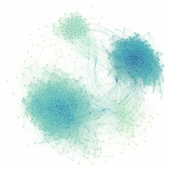
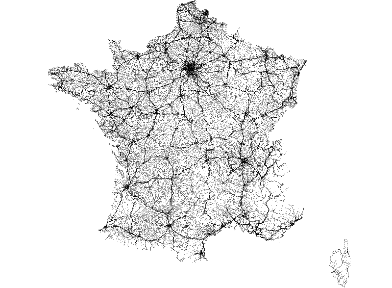
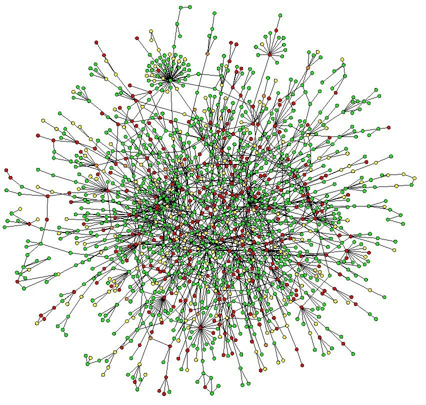
Graphs are ubiquitous
they evolve over time
many of them share a common feature:
Social
Biological
Transport

P2P
....
Overview of the Thesis
Evolving Networks
Temporal Graphs
Dynamic Networks with Churn
Main focus:
Part I:
Part II:
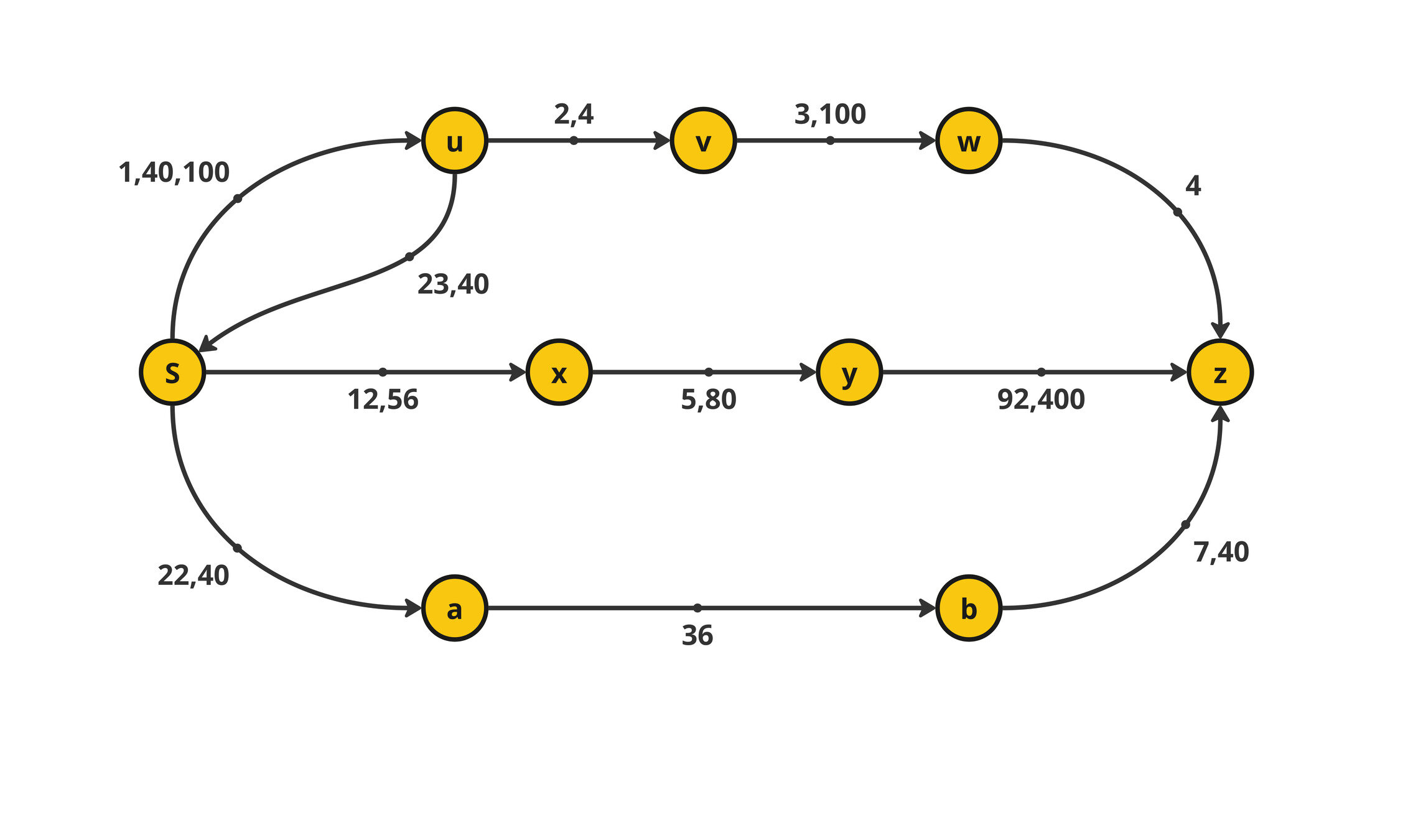
Part IA temporal graph is an ordered triple \(\mathcal{G} = (V,\mathcal{E}, \mathcal{T}) \), where:
- \(V\) is the set of nodes
- \(\mathcal{E}=\{(u,v,t):u,v\in V\land t\in \mathcal{T}\}\) is the set of temporal edges
- \(\mathcal{T} =\{1,2,\dots,T\}\) is a set of time steps
Temporal Graph
Temporal Networks
For each node \(v\in V\)
$$b^{(\star)}_v = \frac{1}{n(n-1)}\sum_{\substack{s, z\in V\\ s\neq z\neq v}} \frac{\sigma^{(\star)}_{s,z}(v)}{\sigma^{(\star)}_{s,z}}\in [0,1]$$
- \(\sigma^{(\star)}_{s,z}(v)\) is the number of \((\star)\)-temporal paths between \(s\) and \(z\) passing through \(v\)
- \(\sigma^{(\star)}_{s,z}\) overall number of \((\star\))-temporal paths between \(s\) and \(z\)
- \((\star)\) can be :
- Shortest
- Shortest-Foremost
- Prefix-Foremost
#P-Hard :(
\(\mathcal{O}(|V|^3|\mathcal{T}|^2)\)
\(\mathcal{O}(|V| |\mathcal{E}|\log |\mathcal{E}|)\)
\(\mathcal{O}(|V||\mathcal{T}|+|\mathcal{E}|)\)
\(\mathcal{O}(|V| + |\mathcal{E}|)\)
Time
Space
- Fastest
- Foremost
Temporal Betwenness [Bu\(\text{\ss}\) et. al, KDD 2020]
Modus operandi to tackle graph mining problems
Step 1 (explorative step)
Can I find a nice heuristic to ``approximate`` such a centrality measure?
Step 2 (ideal step)
Can I design a good approximation algorithm ?
Can be computed in \(\mathcal{O}(M\log M) = \tilde{\mathcal{O}}(M)\) time using \(\mathcal{O}(n+m)\) space
Pass Through Degree (PTD)
\(v\)
\(u\)
\(w\)
\(x\)
\(y\)
\(z\)
\(34\)
\(50\)
\(20\)
\(10\)
\(78\)
\(\text{t-ptd}(v) = \sqrt{|\{(u,w)\in (V\setminus \{v\})^2\}|: u\rightarrow v\rightarrow w\}|}\)
[Becker et al. SEA 2023]
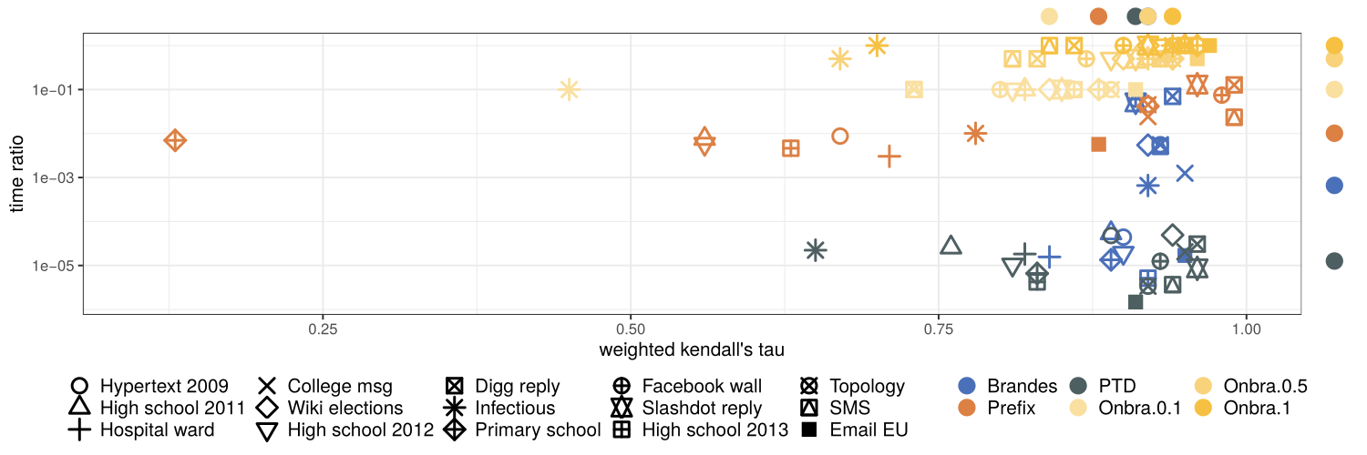
Median w. Kendalls' \(\tau\)
Median time ratio (proxy/exact)
Summary of the experiments
- PTD does not perform worse than the other algorithms
- Faster than all its competitors
- At least as good as ONBRA on 10 over 15 networks
Approximating TBC through Sampling
[Cruciani ECML-PKDD 24]
$$\textbf{Pr}\left(\sup_{v\in V} \left|b_v^{(\star)}-\tilde{b}_v^{(\star)}\right|\leq \varepsilon\right)\geq 1-\delta$$
- Methods are based on random sampling to estimate the temporal betweenness centrality with an acceptable accuracy
-
Problem definition:
- given \(\varepsilon,\delta \in (0,1)\) compute \((\varepsilon,\delta)\)-approximation set \(\tilde{\mathcal{B}}^{(\star)} =\{\tilde{b}_v^{(\star)}:v\in V\}\) such that

Sample Size for \((\varepsilon,\delta)\)-approximation
Vapnik–Chervonenkis (VC) Dimension
\(\displaystyle r = \frac{0.5}{\varepsilon^2} \left(\lfloor \log D^{(\star)}-2\rfloor+1+\ln\left(\frac{1}{\delta}\right)\right)\)
\(\displaystyle r\in \mathcal{O}\left(\frac{\hat{v}+\varepsilon}{\varepsilon^2}\ln\left(\frac{\rho^{(\star)}}{\delta\hat{v}}\right)\right) \)
Variance-Aware
- \(\max_{v\in V}\textbf{Var}(\tilde{b}^{(\star)}_v) \leq \hat{v}\)
- \(\rho^{(\star)} = \displaystyle \frac{1}{n(n-1)}\sum_{s,z\in V}\left|\textbf{Int}(tp_{sz})\right| \)
Where:
- \(D^{(\star)}\) number of nodes in the ``longest'' opt. temporal path
Fast approximation of characteristic quantities
Very high-level idea
With a sample of \(k=\Theta\left(\frac{\ln n}{\varepsilon^2}\right)\) nodes, we can approximate w.h.p.
- \(\rho^{(\star)}\) with the absolute error bounded by \(\varepsilon \frac{D^{(\star)}}{\zeta}\)
- \(D^{(\star)}\) with the absolute error bounded by \(\frac{\varepsilon} {\zeta}\)
- \(\zeta\) with the absolute error bounded by \(\varepsilon\)
Perform \(k\) \((\star)\)-Temporal BFS from random nodes
Temporal Connectivity Rate
Theorem:
MANTRA in three lines
- MANTRA quickly \(\text{\color{blue}``observes''}\) the temporal graph.
- MANTRA starts sampling, computing the approximation as it goes.
- At predefined intervals, MANTRA checks two stopping conditions to understand, using the sample, whether the current approximation has the desired quality.
MANTRA: an \((\varepsilon,\delta)\)-approximation algorithm


Part IISynchronous.
All nodes follow the same clock. In each round \(r=1,2,\dots\)
- Each node sends/receives \(polylog(n)\) messages per round
- Message size \(polylog(n)\)
- Nodes perform local computations
Adversarial Dynamism
An oblivious adversary (knows algorithm, but not the coin toss outcomes) designs churn
\(\mathcal{G} = (G^0,G^1,\dots G^r,\dots)\)
Stochastic Dynamism
The churn follows a stochastic process (a.k.a. Dynamic Random Graph)
Dynamic Networks with Churn (DNC) Model
Expansion and Flooding time on Dynamic Random Regular Expanders
At each round, each node \(u \in V\), independently of the other nodes:
-
If \(deg(u) < d\), then connects to \(d-deg(u)\) new nodes.
-
If \(deg(u) > c\cdot d\), then \(u\) drops \(deg(u) -(c\cdot d)\) neighbors u.a.r.
-
Every edge disappears with probability \(p\).
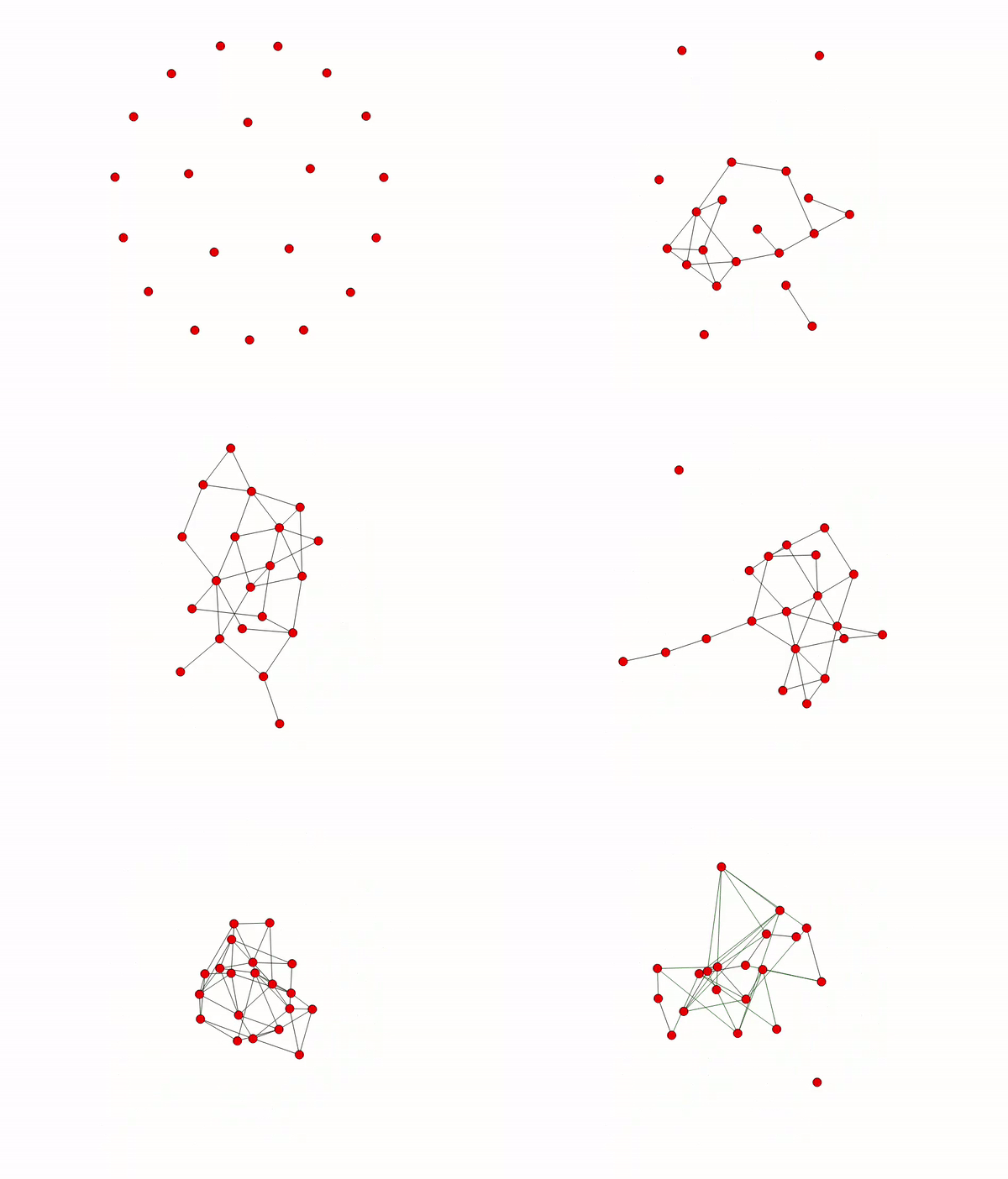
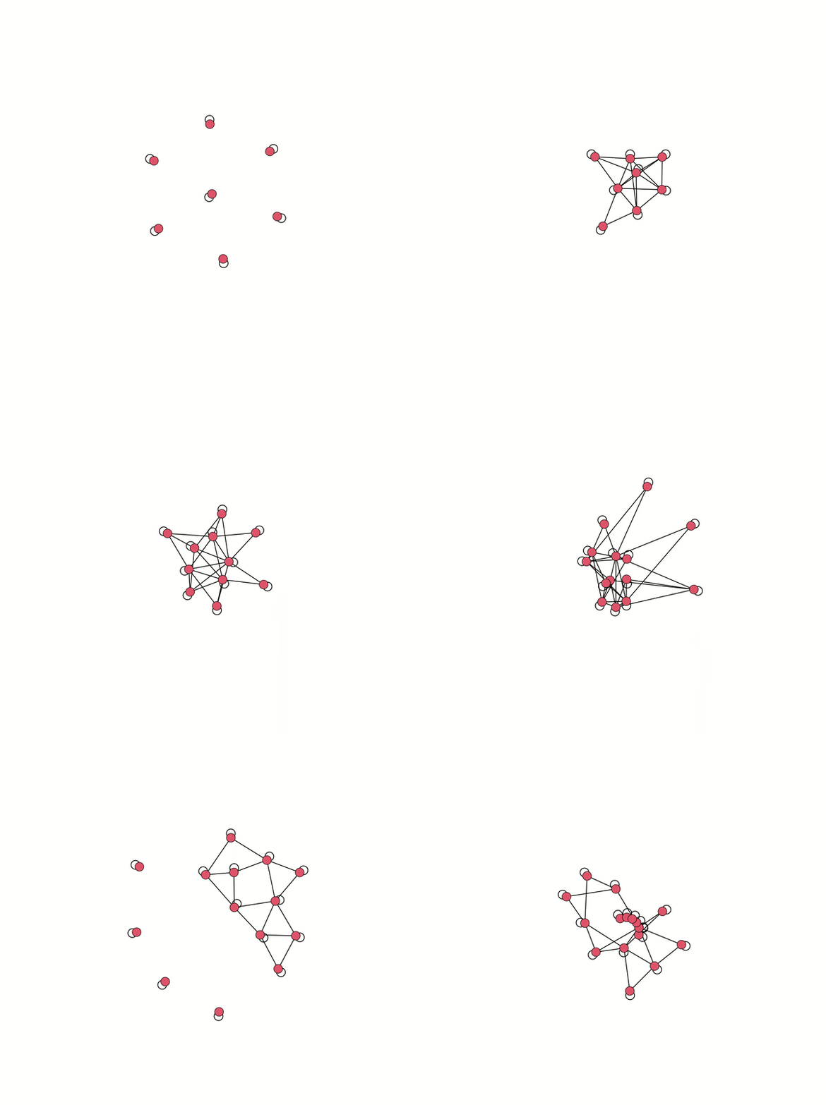
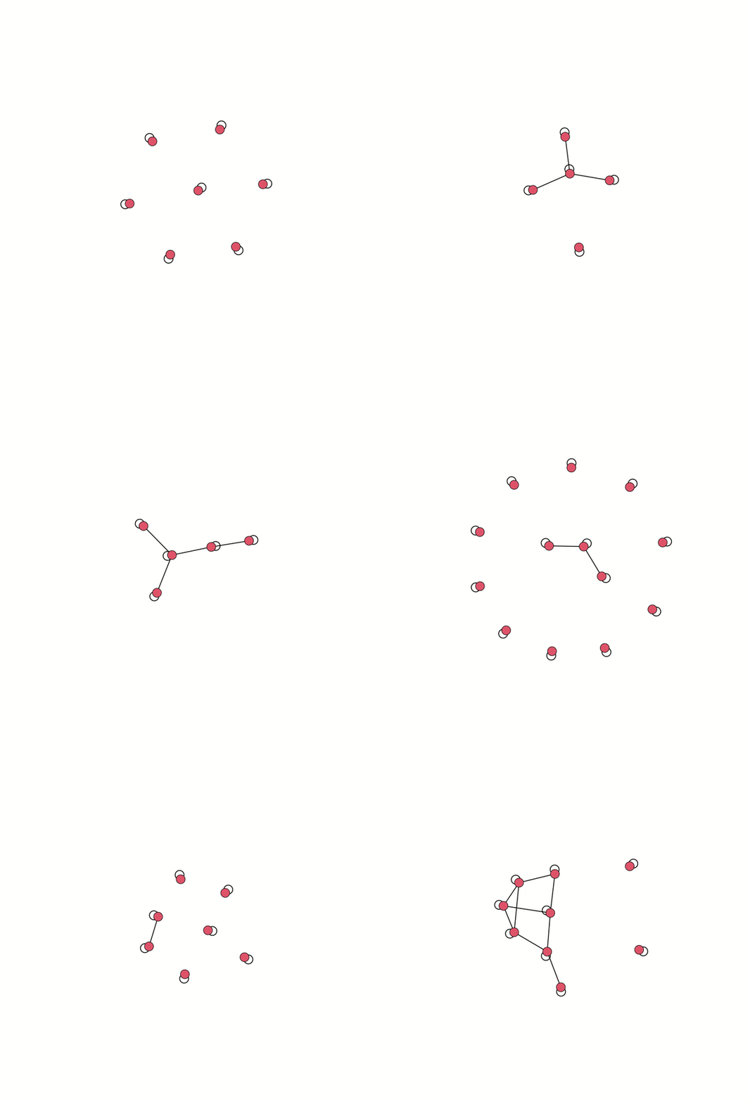
At each round \(t\geq 0\):
- \(N_\lambda(t)\sim \text{Poisson}(\lambda)\) young nodes join the graph and connect to \(d\) random old nodes.
- If an old node \(u\) has \(deg(u) < d\), then connects to \(d-deg(u)\) additional old nodes.
- If an old \(u\) has \(deg(u) > c\cdot d\), then \(u\) drops \(deg(u) -(c\cdot d)\) neighbors u.a.r.
- Every (young and old) node disappears with probability \(q\).
At each round \(t\geq 0\):
- \(N_\lambda(t)\sim \text{Poisson}(\lambda)\) young nodes join the graph and connect to \(d\) random old nodes.
- If an old node \(u\) has \(deg(u) < d\), then connects to \(d-deg(u)\) additional old nodes.
- If an old \(u\) has \(deg(u)> c\cdot d\), then \(u\) drops \(deg(u) -(c\cdot d)\) neighbors u.a.r.
- Every (young and old) node disappears with probability \(q\).
- Every edge disappears with probability \(p\).
We observe:
- Good Expander Graph at each time step
- Logarithmic Flooding Time (# Rounds to spread information from a node)
[Cruciani and Pasquale
ICDCN 23]
A preliminary version of this work appeared as a Brief Ann. in SS 2022.
- Sparse settings (\(d = 4,c=1.5\))
- Highly Dynamic Settings
- All values of \(n\)
All the results hold also for:
Maintaining Distributed Data Structures in Dynamic Peer-to-Peer Networks
[Augustine et al., ArXiv]
Adversarial Churn.
Stable Network Size.
Up to \(\mathcal{O}(n/\log n)\) nodes leave/join the network per round.
Number of nodes \(n\) unchanged over time
(In each round: # churned out = #churned in)
Can be relaxed!
Connectivity assumption.
The adversary cannot connect all the new nodes to only one peer in the network
Our Problem
- Build and maintain a data structure despite the churn
- Data structure must be queryable at each round
- Each node in the overlay has one element in the DS
- The maintaning algorithm must be efficient
Dynamic Resource Competitiveness
Our distributed algorithm must be efficient
Workload: #Created Edges + #Messages
\(t_{start}-\alpha\)
\(\alpha = \mathcal{O}(\log n)\)
\(\beta = polylog(n)\)
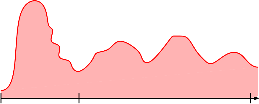
Churn

Workload \(\leq\beta\cdot\)Churn(\(t_{start}-\alpha,t_{end}\))
\(t_{start}\)
\(t_{end}\)
Skip List

H
H
T
\(-\infty\)
\(\infty\)
\(22\)
\(56\)
\(78\)
\(79\)
\(83\)
\(97\)
Tail
Head
LV. 0
LV. 1
LV. 2
Is \(83\) in the SL. ?
Let's decouple the
data structure
from the overlay network
Our Idea
The Maintenance Cycle

1
2
3
4

Overlay Network
Clean Network
Buffer Network
Live Network
Committee
Clique of \(\Theta(\log n)\) random nodes
Main Result
- Can be extended to skip graphs
- Works with multiple keys on each node of the overlay
- Can build and maintain a skip list despite heavy churn
- \(\mathcal{O}(\log n)\) rounds maintenance algorithm
- Algorithm's workload is proportional to the experienced churn
- The skip list is maintained for \(n^c, (c\geq 1)\) rounds w.h.p.
Conclusion
Part I
Part II
- Introduced a novel temporal degree notion and experimentally compared several heuristics to approximate the shortest temporal betweenness rankings
- Introduced MANTRA, a novel sampling-based approximation algorithm for the temporal betweenness centrality
- Provided a sample-complexity analysis for the temporal betweenness estimation problem
- Provided a sampling-based approximation algorithm for temporal distance-based metrics in temporal graphs
- Proposed several Dynamic Random Graphs and empirically studied their properties
- Provided a distributed protocol that builds and maintains a distributed skip list despite a heavy adversarial churn
Thank You
-
[Becker, Crescenzi, C, Kodric] Proxying Betweenness Centrality Rankings in Temporal Networks (SEA 2023)
- [Cruciani] MANTRA: Temporal Betweenness Centrality Approximation through Sampling (ECML-PKDD 2024)
- [Augustine, C, Gillani] Maintaining Distributed Data Structures in Dynamic Peer-to-Peer Networks. (2024, Available on ArXiv )
- [ C, Pasquale] Dynamic graph models inspired by the Bitcoin network-formation process (ICDCN 2023 - BA: SSS 2022)
- [Augustine, C, Kumar, Kutten, Peleg] Partial Gossip in an Anonymous Node-Capacitated Clique (2024, Submitted).
- [ C, Pellegrina] Fast Estimation of Percolation Centrality (2024, Available on ArXiv)
- [ C, Pellegrina] Fair Centrality Maximization (Working Paper)
-
[Amati, C, Pasquini, Vocca, Angelini] PROPAGATE: a seed propagation framework to compute Distance-based metrics on Very Large Graphs (ECML-PKDD 2023)
- [Augustine, C, Götte] Maintaining Overlays Under Adversarial Churn (Working Paper)
- [Chatterjee, C, Kumar] FOX: Fast Construction of Expanders (Working Paper)
-
[C, Pasquini, Amati, Vocca, Angelini] FESTER: Fast Approximation of Geometric Centralities on Very Large Graphs (Working Paper)
Overview of my research
Additional Experiments for
Proxies
Why PTD?
Existing temporal degree definitions:
- Degree on the underlying graph: \(d_{und}(v) = \left| \bigcup_{t\in[T]}N_t(v)\right|\)
- Average degree [Latapy (2018)]: \(d_{avg}(v) =\frac{1}{|T|}\sum_{t\in[T]}|N_t(v)|\)
\(d_{und}(v)\)
\(d_{avg}(v)\)
\(\text{t-ptd}(v)\)
\(k+1\)
\(1\)
\(\sqrt{k}\)
\(1\)
\(1\)
\(1\)
\(k+1\)
\(1\)
\(\sqrt{\frac{k(k+1)}{2}}\approx k\)
Where \(N_t(v) = \{u\in N(v):(v,u,t)\in \mathcal{E}\}\)
\(v\)
$$1,2,...,k+1$$
\(v\)
$$1$$
$$2$$
$$2$$
\(v\)
$$1$$
$$2$$
$$k+1$$
1) Brandes' Algorithm algorithm on the underlying graph
2) Prefix foremost-temporal betweenness algorithm
\(\mathcal{O}(n M \log M )\)
3) ONBRA [Santoro & Sarpe, WWW 2022]
\(\mathcal{O}(s \cdot T\cdot \log (n\cdot T) )\)
\(\mathcal{O}(n m )\)
- \(t(\text{ONBRA}) = t(\text{Exact})/2 \)
- \(t(\text{ONBRA}) = t(\text{Exact})/10 \)
- \(t(\text{ONBRA}) = t(\text{Exact}) \)
Global proxies
Datasets
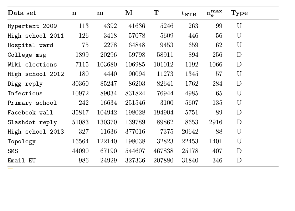
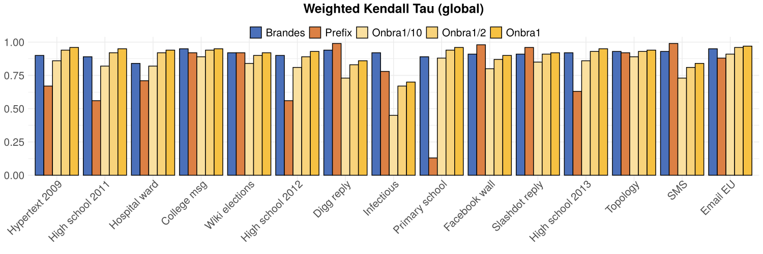
Brandes
Prefix
ONBRA 1
W. Kendall's \(\tau\)
3
5
10
ONBRA \(\frac{1}{10}\)
0
11
# times a proxy wins
Experiment: Global Proxies rank correlation
Brandes
Prefix
ONBRA 1
W. Kendall's \(\tau\)
3
5
10
ONBRA \(\frac{1}{10}\)
0
11
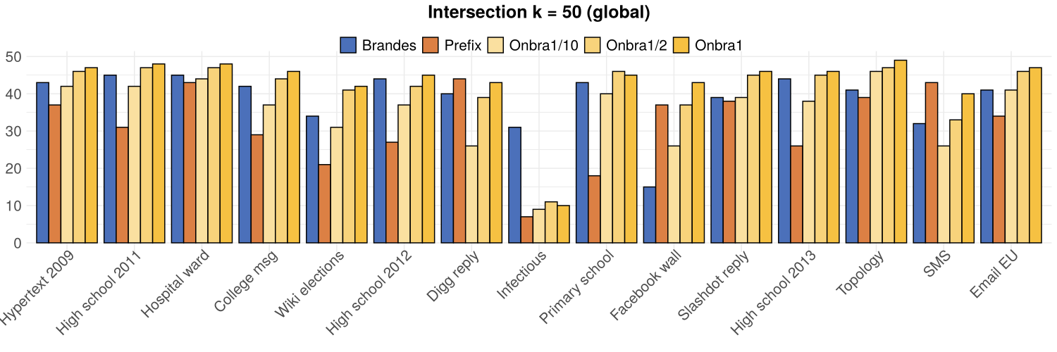
TOP(50)
2
1
12
11
3
3
# times a proxy wins
Experiment: Global Proxies rank correlation
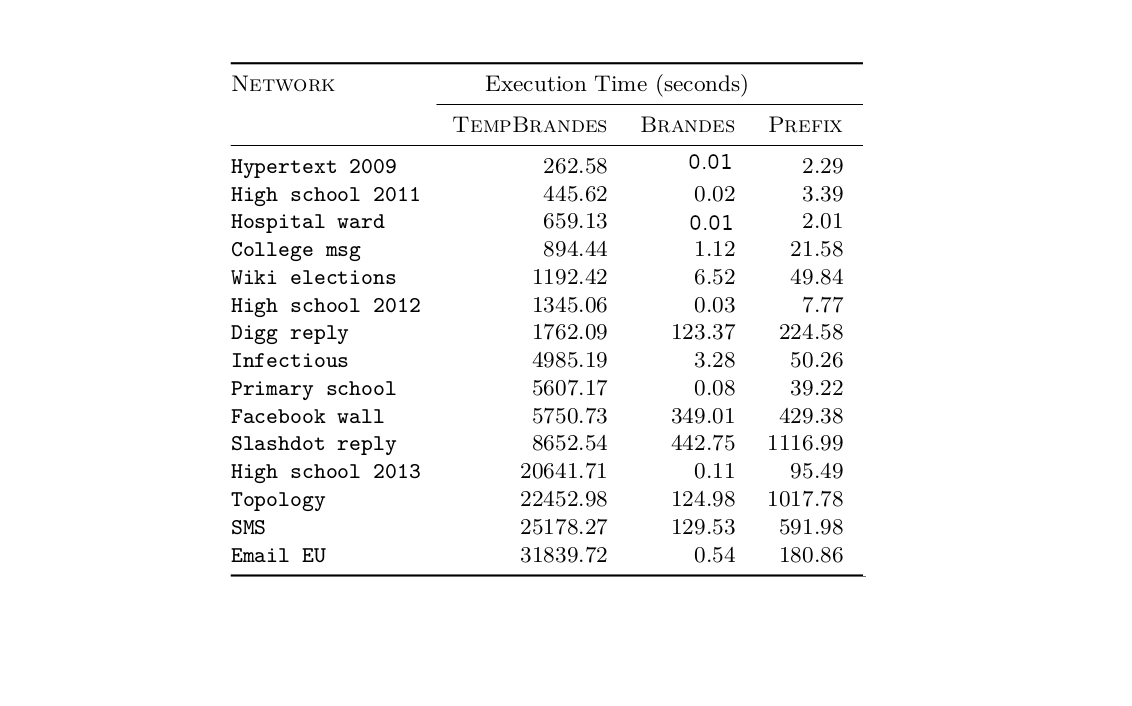
Experiment: Running time
Experiments: local proxy rank correlations
W. Kendall's \(\tau\)
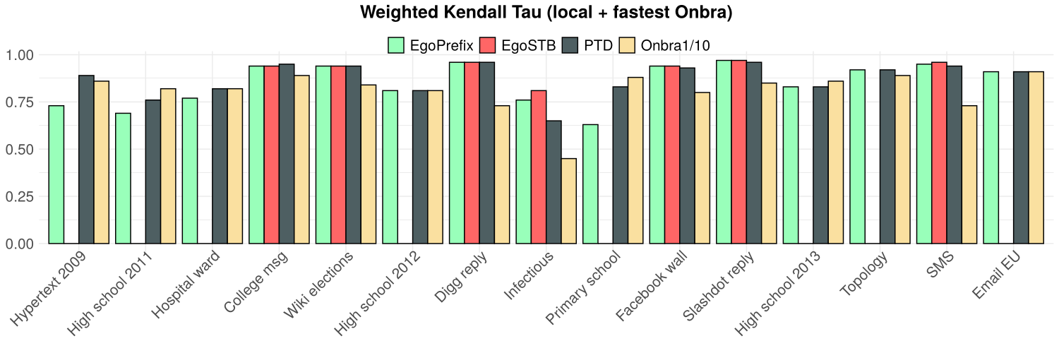
- PTD does not perform worse than EgoSTB and ONBRA
- At least as good as ONBRA on 10 over 15 networks
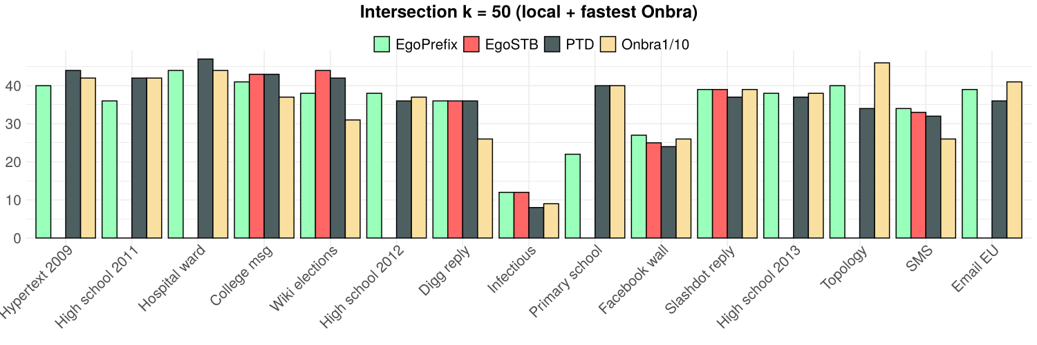
and TOP(50)
Running Times
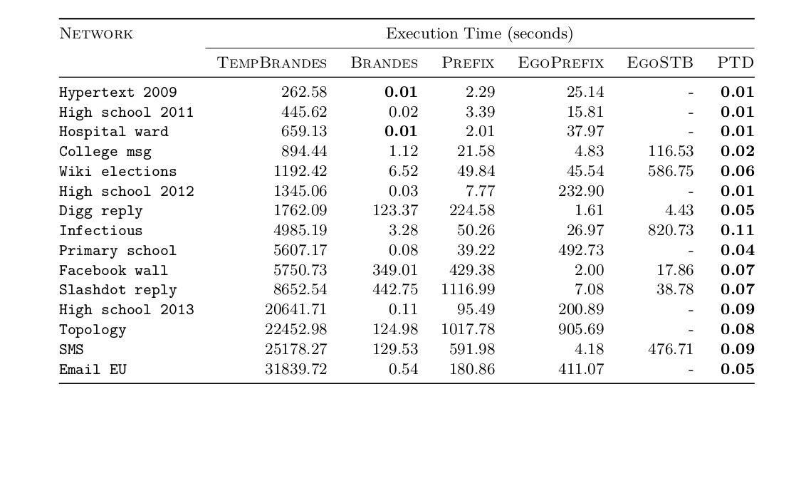
Additional Experiments for
MANTRA
Experimental Setting

All the algorithms have been implemented in Julia
Every algorithm is run 10 times
\(\delta = 0.1\)
\(\varepsilon\in\{0.1,0.07,0.05,0.01,0.007.0.005,0.001\}\)
Parameters:
\(c = 25\)
Machine used: Server with Intel Xeon Gold 6248R (3.0GHz)
32 cores and 1TB RAM (@CyStar group at IITM)
Temporal Networks

Temporal Networks: properties

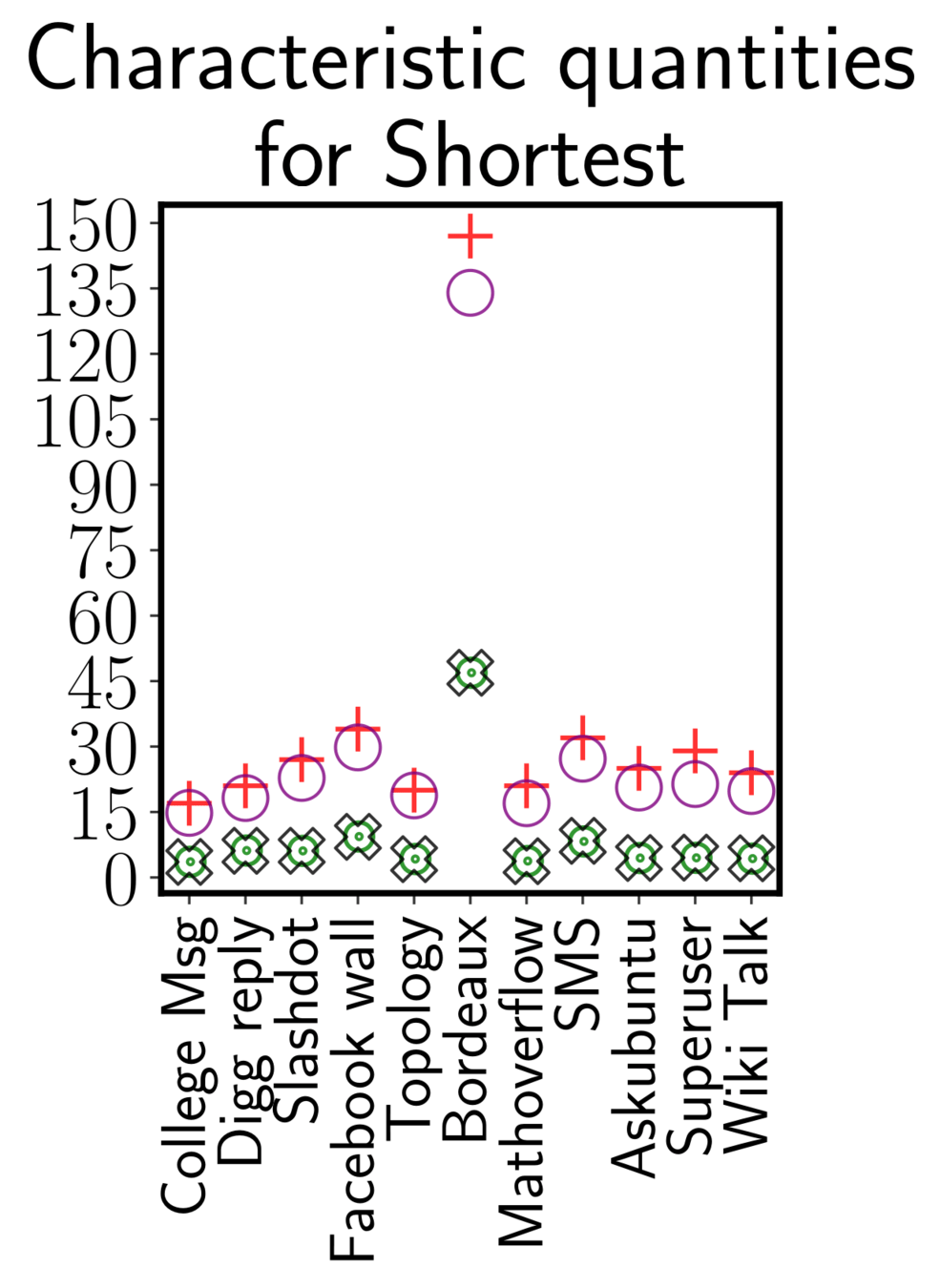

Running time sampling algorithm
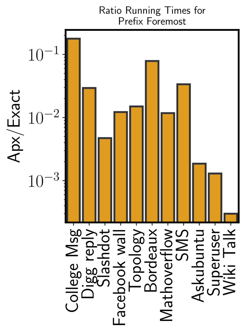
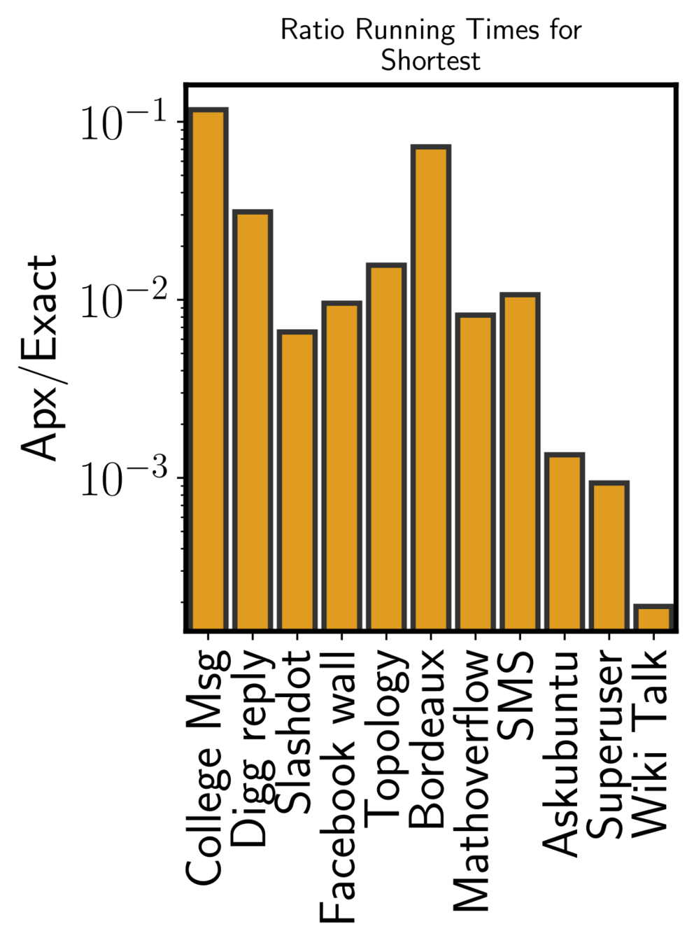
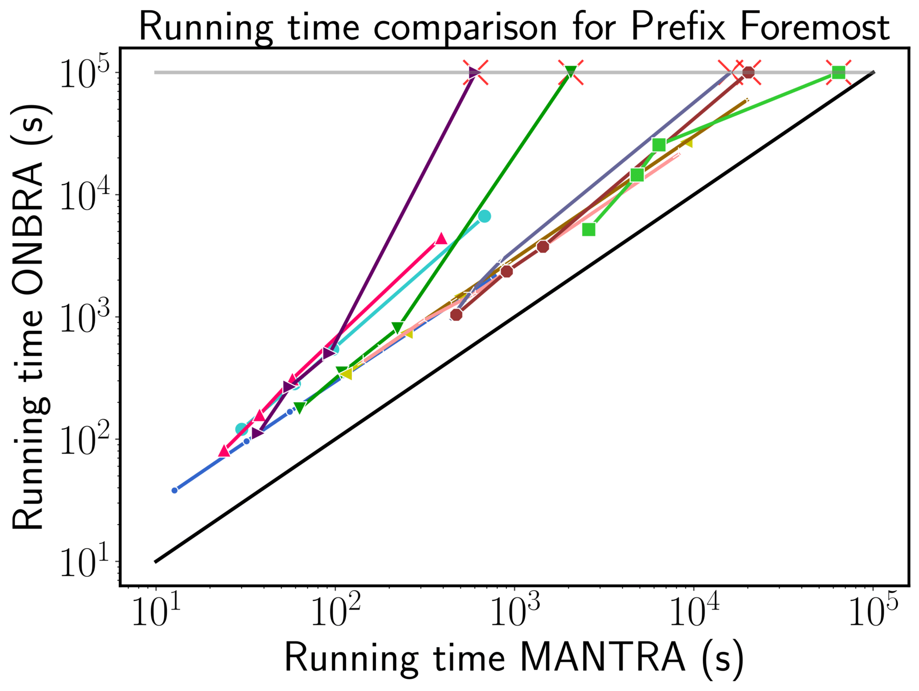
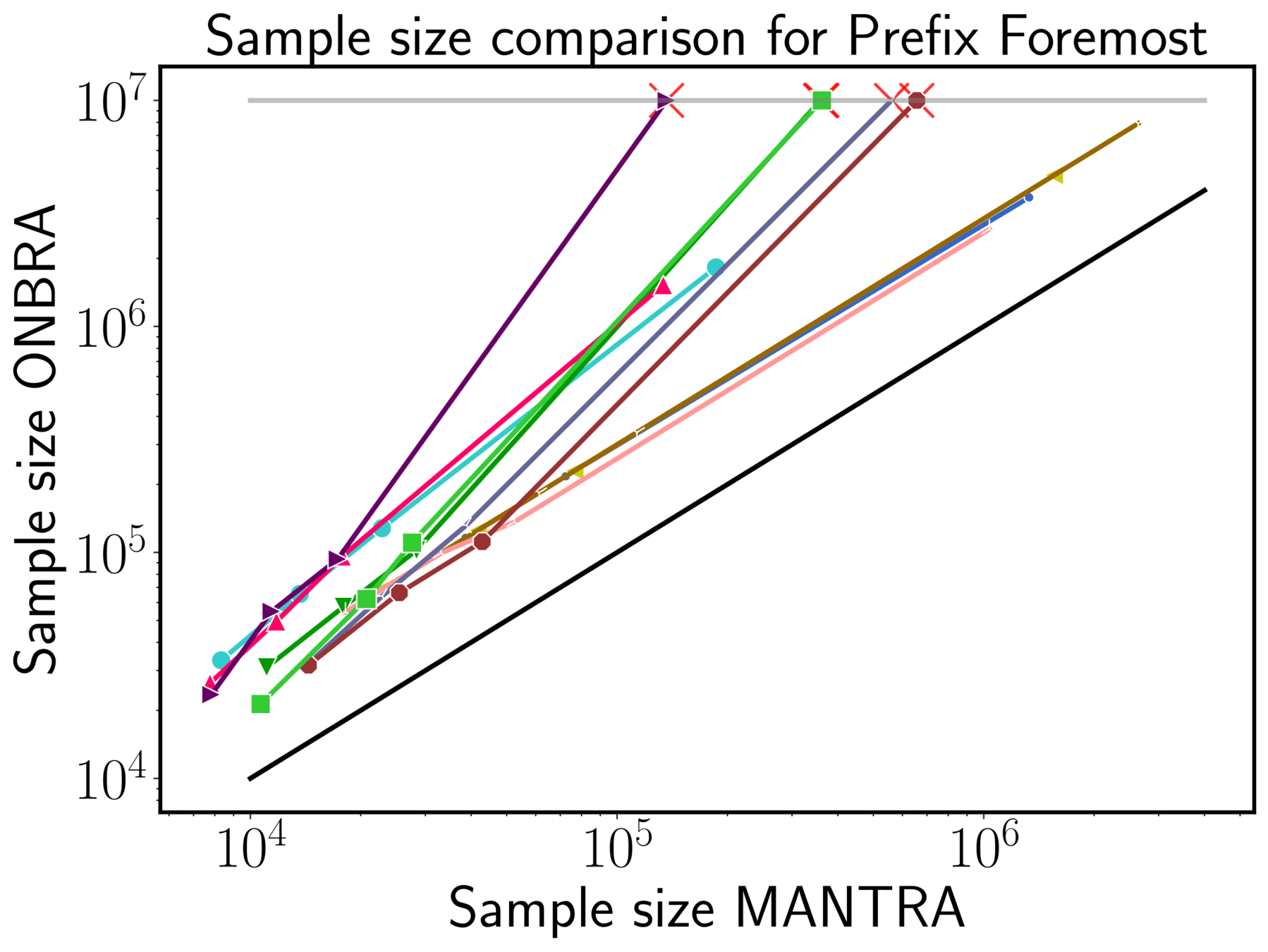
MANTRA vs ONBRA (sh)
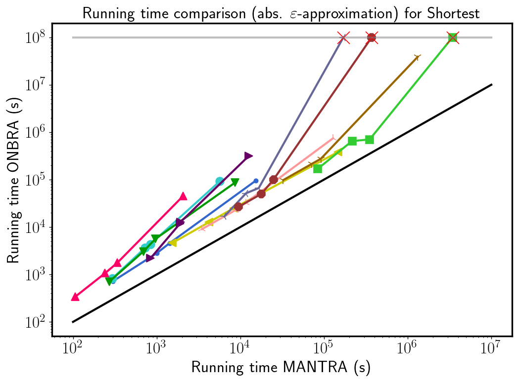

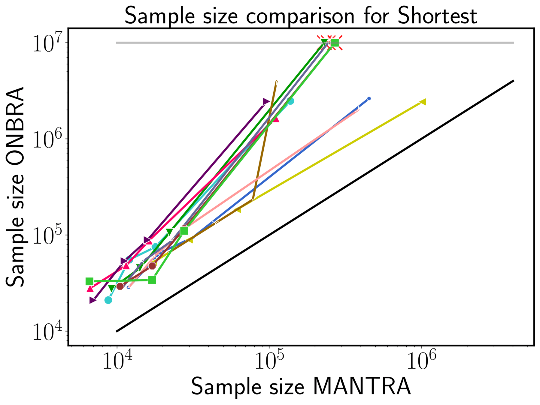

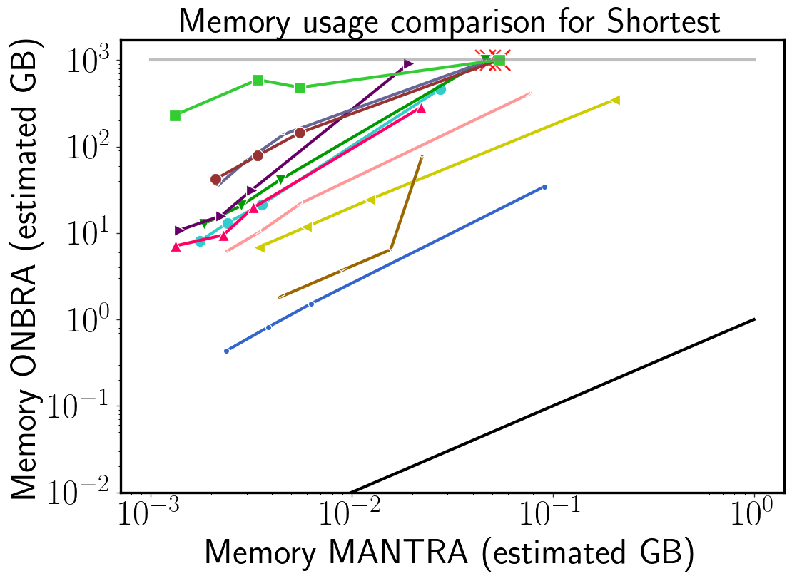
MANTRA vs ONBRA (sh)
MANTRA
Progressive Sampling
Sampling Algorithm
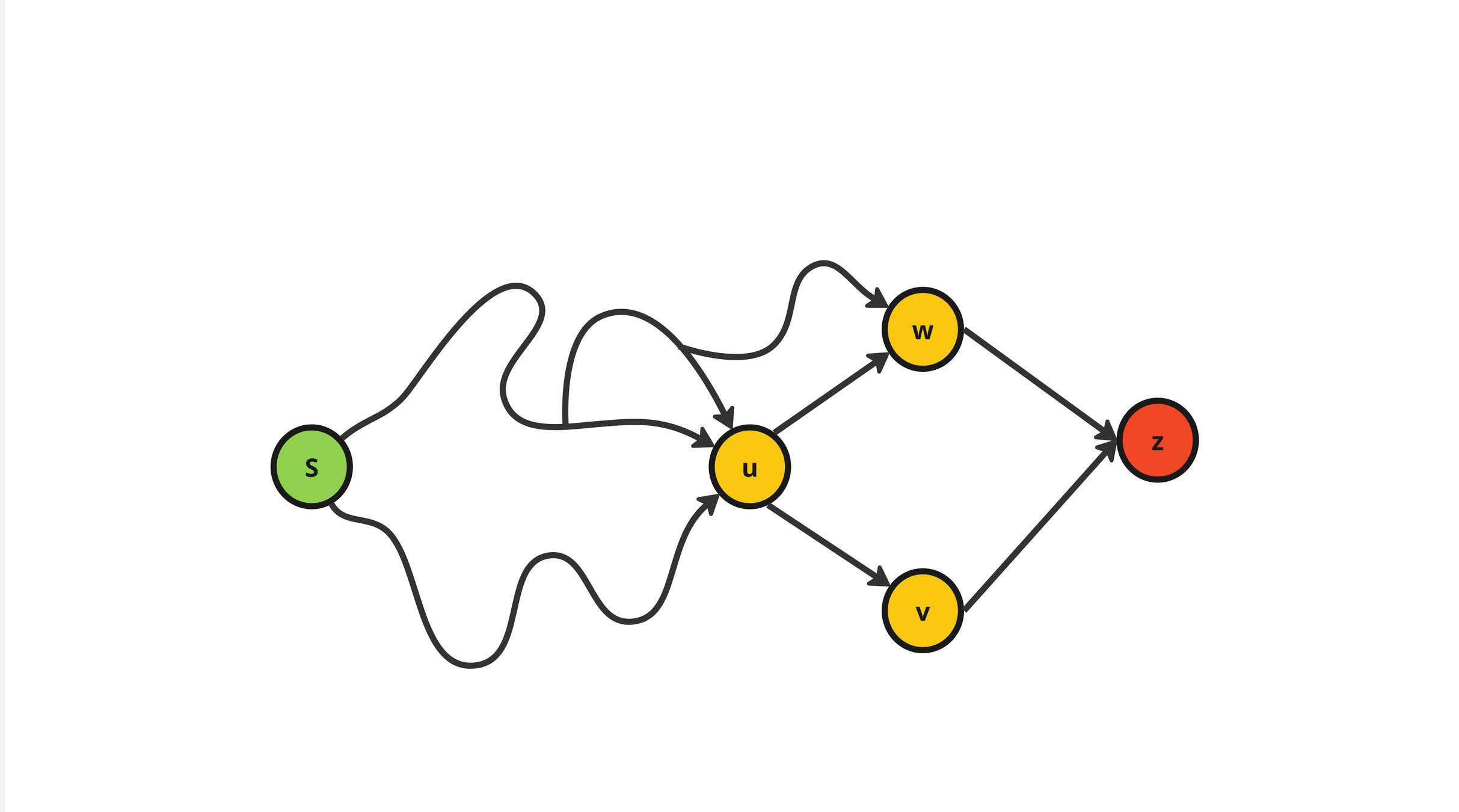
s
z
\(f_u(s,z) =\frac{\sigma^{(\star)}_{s,z}(u)}{\sigma^{(\star)}_{s,z}}\)
\(f_v(s,z) =\frac{\sigma^{(\star)}_{s,z}(v)}{\sigma^{(\star)}_{s,z}}\)
\(f_w(s,z) =\frac{\sigma^{(\star)}_{s,z}(v)}{\sigma^{(\star)}_{s,z}}\)
MANTRA
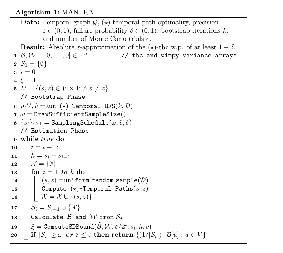


Bootstrap Phase
Estimation Phase
Sample Size for \((\varepsilon,\delta)\)-approximation
Theorem:
Given a temporal graph \(\mathcal{G}\), the parameters \(\varepsilon,\delta\in (0,1)\) and a sample \(\mathcal{S}\) of size \(r\)
MANTRA computes an \((\varepsilon,\delta)\)-approximation of the
- Shortest (foremost/fastest) TBC in time \(\widetilde{\mathcal{O}}(r\cdot n\cdot T)\)
- Prefix Foremost TBC in time \(\widetilde{\mathcal{O}}(r\cdot M)\)
Using \(\mathcal{O}(n+M)\) space.
Supremum Deviation
Given a set of functions \(\mathcal{F}\) from a domain \(\mathcal{D}\) and a sample \(\mathcal{S}\)
$$\textbf{SD}(\mathcal{F},\mathcal{S}) =\sup_{f\in \mathcal{F}}{\left| a_f(\mathcal{S})-\mu_f\right|} $$
Text
$$a_f(\mathcal{S}) = \frac{1}{|\mathcal{S}|} \sum_{i = 1}^{|\mathcal{S}|}f(s_i) $$
$$\mu_f = \mathbb{E}[a_f(\mathcal{S})] $$
The Supremum Deviation
Goal:
$$\textbf{SD}(\mathcal{F},\mathcal{S})$$
To find an Upper bound for
Rademacher Averages
Text
c-Monte Carlo Emprical Rademacher Averages (c-MCERA)
$$\bm{\lambda} \in \{-1,+1\}^{c\times|\mathcal{S}|}, r = |\mathcal{S}|$$
$$R^c_{r}(\mathcal{F},\mathcal{S},\bm{\lambda}) = \frac{1}{c}\sum_{j=1}^c \sup_{f\in\mathcal{F}}\frac{1}{r} \sum_{s_i\in\mathcal{S}}\lambda_{j,i} f(s_i) $$
With Probability at least
$$1-\delta$$
$$\mathcal{W}_\mathcal{F}(\mathcal{S})= \sup_{f\in \mathcal{F}} \frac{1}{r}\sum_{s_i\in\mathcal{S}}(f(s_i))^2$$
Empirical
Wimpy Variance
\(R = \tilde{R} + \frac{\ln(4/\delta)}{r}+\sqrt{\left(\frac{\ln(4/\delta)}{r}\right)^2 + \frac{2\ln(4/\delta)\tilde{R}}{r}}\)
\(\xi = 2R + \sqrt{\frac{2 \ln(4/\delta)\left(\hat{v}+4R\right)}{r}}+\frac{\ln(4/\delta)}{3r}\)
$$\textbf{SD}(\mathcal{F},\mathcal{S})\leq \xi$$
Variance Dependent Bound
\(\tilde{R} = R^c_{r}(\mathcal{F},\mathcal{S},\bm{\lambda}) + \sqrt{\frac{4 \mathcal{W}_{\mathcal{F}}(\mathcal{S})\ln(4/\delta)}{cr}}\)
Back to the Temporal Betweenness
\(f_v(s,z) =\frac{\sigma^{(\star)}_{s,z}(v)}{\sigma^{(\star)}_{s,z}}\)
\(\mathcal{D} = \{(s,z)\in V\times V : s\neq z\}\)
$$\tilde{b}^{(\star)}_v =\frac{1}{|\mathcal{S}|}\sum_{(s,z)\in \mathcal{S}} f_v(s,z) $$
Functions
Domain
Sample Mean
$$\mathcal{W}_\mathcal{F}(\mathcal{S})= \sup_{v\in V} \frac{1}{|\mathcal{S}|}\sum_{(s,z)\in\mathcal{S}}(f_v(s,z) )^2$$
Emp. Wimpy Variance
Expansion and Flooding time on Dynamic Random Regular Expanders
Average Flooding Time: Sparse vs Dense
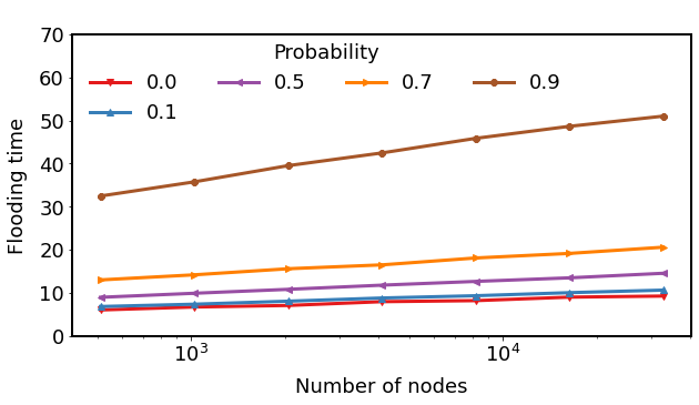
\(d : 4, c: 1.5\)
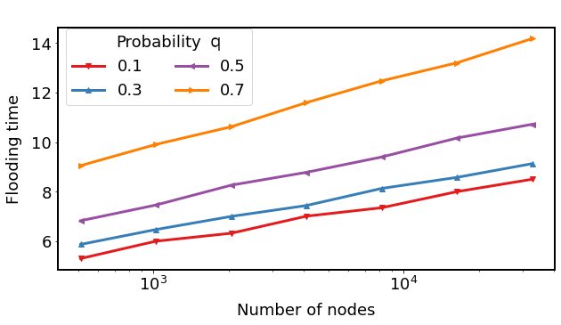
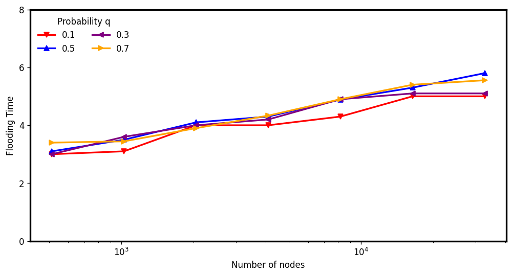
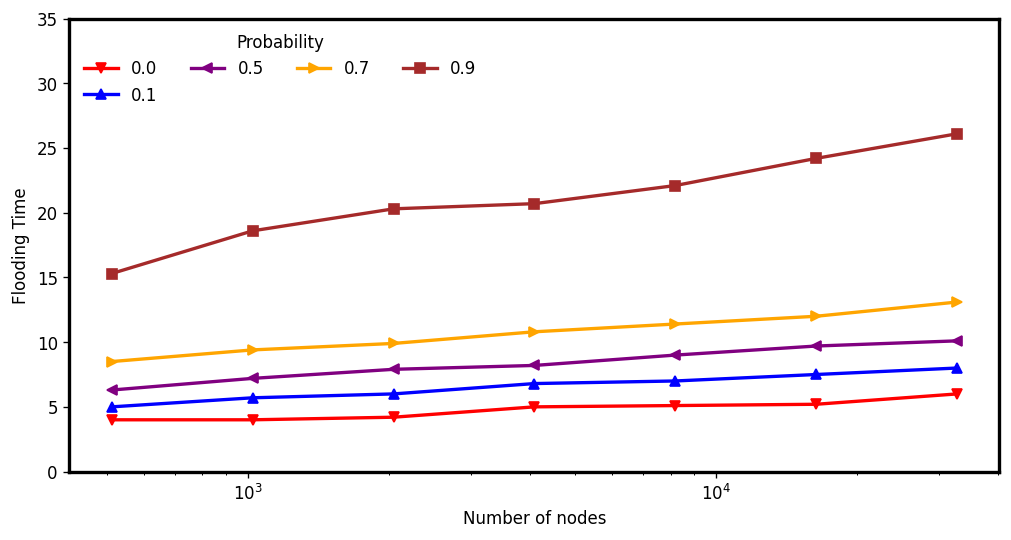
\(d : 6, c: 5\)
Vertex-Dynamic
Edge-Dynamic
$$(n = 2^{15})$$
Average Flooding Time: Sparse vs Bitcoin Default values
Edge & Vertex-Dynamic
$$(n = 2^{15})$$

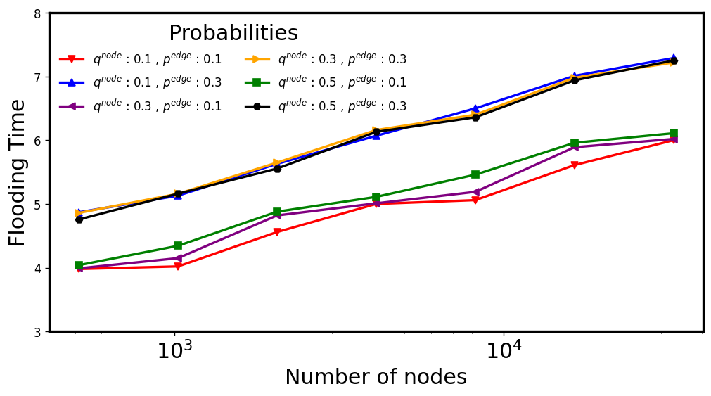
\( d: 4, c: 1.5\)
\(q\in [0.1,0.5],p\in [0.1,0.3] \)
\( d: 8, c: 15.625\)
\(q\in [0.1,0.5],p\in [0.1,0.3] \)
Dynamic Distributed
Data Structures
Dynamic Resource Competitiveness
Our distributed algorithm must be efficient
Workload: #Created Edges + #Messages
\(t_{start}-\alpha\)
\(\alpha = \mathcal{O}(\log n)\)
\(\beta = polylog(n)\)

Churn

Workload \(\leq\beta\cdot\)Churn(\(t_{start}-\alpha,t_{end}\))
\(t_{start}\)
\(t_{end}\)
Overview of the Cycle

Spartan: The Overlay Network
0
1
0
0
1
2
3
Level
Row
Committee
Committee:
- Clique of \(\Theta(\log n)\) random nodes
- Nodes randomly change committee
- Cannot be destroyed w.h.p
Augustine et. al [J.P.D.C. 2021]
Dealing with the nodes removed by the adversary
Gets removed
Gets replaced by committee
''Virtual node''
Deletion Phase
\(a\)
\(b\)
\(c\)
\(d\)
\(e\)
\(f\)
\(g\)
\(h\)
\(i\)
\(j\)
\(\infty\)
\(-\infty\)
We can delete all the virtual nodes in \(\mathcal{O}(\log n)\) rounds w.h.p
- Tree Formation
- Propagation
\(\mathcal{O}(\log n)\) w.hp.
\(\mathcal{O}(\log n)\) w.h.p.
\(k\)
\(\ell\)
\(f\)
Buffer Creation Phase
We can create the Buffer in \(\mathcal{O}(\log n)\) rounds!
Ajtai, Komlós, and Szemeréd (AKS) Network [STOC, 1983]
How? Using sorting networks
3
4
2
1
Input
Output
3
4
1
2
1
3
4
2
1
2
3
4
What sorting network?
How can we use it?
Maggs et al. [Algorithmica, 2000]
Can be efficiently simulated on multibutterfly networks!
Buffer Creation:
1. Build a multibutterfly \(\mathcal{M}\)
2. Run AKS on \(\mathcal{M}\)
3. Build the upper level of the skip list
\(\mathcal{O}(\log n)\) w.h.p.
\(\mathcal{O}(\log n)\)
\(\mathcal{O}(\log n)\) w.h.p.
# Of Rounds
Buffer Creation Phase
AKS


Merge Phase
We need to merge the Buffer Network with the Clean Network
Can be done in \(\mathcal{O}(\log n)\) rounds w.h.p.
\(\mathcal{O}(n)\)


\(\mathcal{O}(n)\)
\(-\infty\)
\(\infty\)
\(5\)
\(13\)
\(27\)
\(45\)
\(50\)
\(ls\)
\(rs\)
\(1\)
\(23\)
\(25\)
\(55\)
\(98\)
\(-\infty\)
\(\infty\)
\(5\)
\(13\)
\(27\)
\(45\)
\(50\)
\(ls\)
\(rs\)
\(1\)
\(23\)
\(25\)
\(55\)
\(98\)
Buffer Network
Clean Network
Merge Phase: WAVE Protocol
\(-\infty\)
\(\infty\)
\(5\)
\(13\)
\(27\)
\(45\)
\(50\)
\(ls\)
\(rs\)
\(1\)
\(23\)
\(25\)
\(55\)
\(98\)
WAVE Protocol: Down the rabbit hole
\(ls\)
\(rs\)
\(1\)
\(23\)
\(25\)
\(55\)
\(98\)
\(23\)
\(25\)
\(25\)
\(55\)
\(25\)
\(1\)
\(98\)
\(55\)
Parent-Children relationship
WAVE Protocol: Down the rabbit hole
Cohesive Group
Group Leader
Followers
WAVE Protocol: Down the rabbit hole
- The leader of a Cohesive Group is in charge of traversing the target skip list
- Every time the leader moves on the Clean Network:
1. Informs its followers
2. Informs its children
- Every time a follower receive a message:
1. Virtually walks on the Clean Network
2. Informs its children
\(ls\)
\(rs\)
\(1\)
\(23\)
\(25\)
\(55\)
\(98\)
\(-\infty\)
\(\infty\)
\(5\)
\(13\)
\(27\)
\(45\)
\(50\)
\(ls\)
\(1\)
\(23\)
\(25\)
\(1\)
\(ls\)
Some Children
Cohesive Group
\(23\)
\(98\)
\(rs\)
\(ls\)
\(ls\)
\(1\)
\(23\)
\(25\)
\(1\)
\(ls\)
\(23\)
\(98\)
\(rs\)
Some Children
Cohesive Group(s)
\(23\)
\(98\)
\(rs\)
\(ls\)
\(-\infty\)
\(\infty\)
\(5\)
\(13\)
\(27\)
\(45\)
\(50\)
\(ls\)
\(23\)
\(98\)
\(rs\)
\(98\)
\(rs\)
\(25\)
\(55\)
\(1\)
Update Phase
- We need to Update the Live Network with the Clean Network
- Two type of edges:
Present in the Clean Network
Present in both Networks
Our Problem
- Build and maintain a data structure despite the churn
- Data structure must be queryable at each round
Is \(x\) in the DS ?
round \(r\)
Yes
No
If life of the element subsumes \([r,r+Q]\)
If no node \(x\) with effective life-time overlapping \([r,r+Q]\)
DS
\(Q\)
- Each node in the overlay has one element in the DS
- The maintaning algorithm must be efficient
Spartan: The Overlay Network
0
1
0
0
1
2
3
Level
Row
Committee
Committee:
- Clique of \(\Theta(\log n)\) random nodes
- Nodes randomly change committee
- Cannot be destroyed w.h.p
Augustine et. al [J.P.D.C. 2021]
Dealing with the nodes removed by the adversary
Gets removed
Gets replaced by committee
''Virtual node''
\(a\)
\(b\)
\(c\)
\(d\)
\(e\)
\(f\)
\(g\)
\(h\)
\(i\)
\(j\)
\(\infty\)
\(-\infty\)
\(k\)
\(\ell\)
\(f\)
\(a\)
\(c\)
\(d\)
\(e\)
\(f\)
\(g\)
\(h\)
\(\infty\)
\(-\infty\)
\(f\)
Deletion Phase
We can delete all the virtual nodes in \(\mathcal{O}(\log n)\) rounds w.h.p
Buffer Creation Phase
AKS


We can create the Buffer in \(\mathcal{O}(\log n)\) rounds!