Proxying Betweenness Centrality Rankings in Temporal Networks
Ruben Becker Pierluigi Crescenzi
Antonio Cruciani Bojana Kodric

{pierluigi.crescenzi,antonio.cruciani}@gssi.it

{rubensimon.becker,bojana.kodric}@unive.it
Temporal Networks
Graphs are ubiquitous and many of them share a common feature:
they evolve over time
A directed temporal graph is an ordered triple \(\mathcal{G} = ( V,\mathcal{A},T)\), where:
- \(V\) is the set of nodes
- \(\mathcal{A} = \{(u,v,t): u,v\in V\land t\in [T] \}\) is the set of temporal arcs
- \(T = \{1,2,\dots, |T|\}\) is a set of time steps
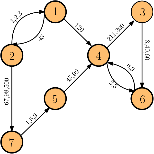

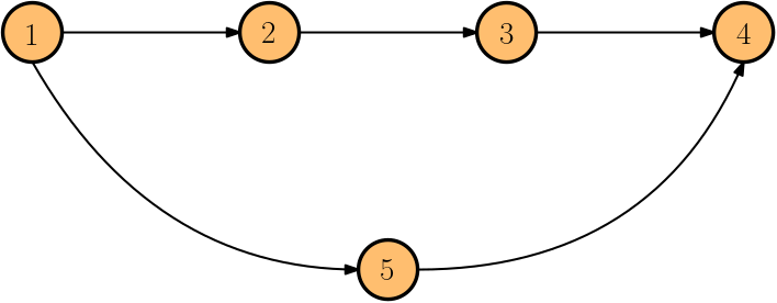
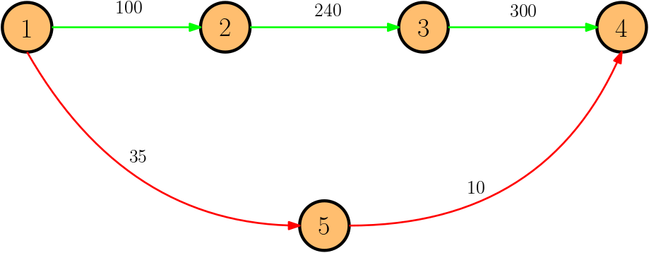
Temporal Graph
Underlying Graph
Temporal Paths
A temporal path is a sequence \(P = \langle (u_1,v_1,t_1),(u_2,v_2,t_2),\dots ,(u_k,v_k,t_k)\rangle\) of temporal arcs in which \(t_i < t_{i+1} \) and \(v_i = u_{i+1}\) for all \(i\in [k-1]\) and each node in \(V\) is visited at most once.
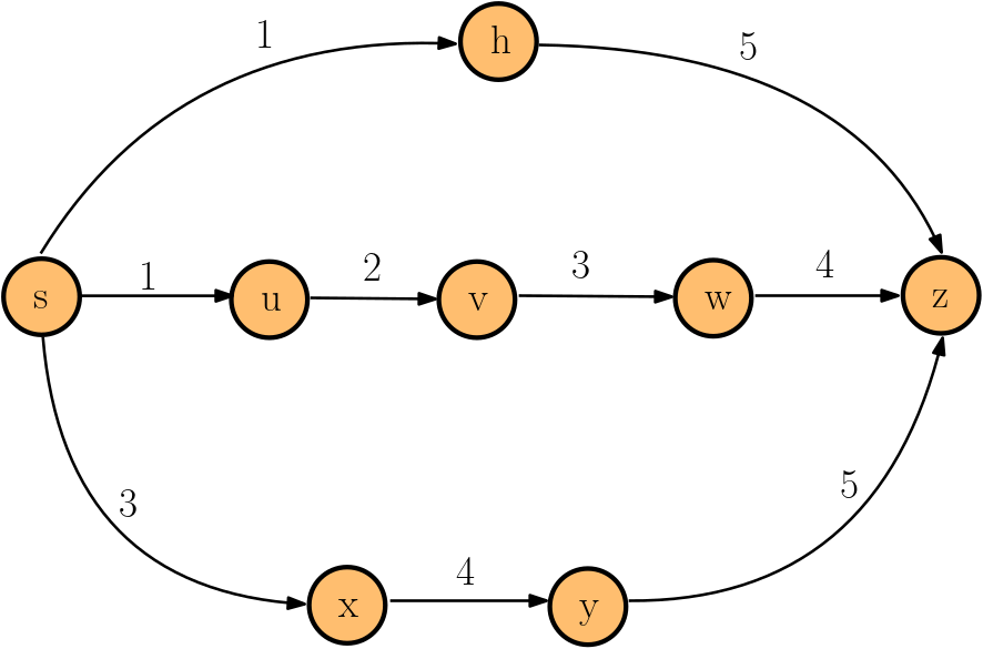
\(P = \langle s \rightarrow h\rightarrow z \rangle \)
Shortest
Foremost
Fastest
\(P = \langle s \rightarrow u \rightarrow v \rightarrow w \rightarrow z \rangle \)
\(P = \langle s \rightarrow x\rightarrow y\rightarrow z \rangle \)
Temporal Betweenness [Bu\(\text{\ss}\) et al (KDD 2020)]
The temporal betweeness centrality of each node \(v\in V\) is defined as
$$tb(v) = \sum_{\substack{s, z\in V\\ s\neq z\neq v}} \frac{\sigma^{(\star)}_{s,z}(v)}{\sigma^{(\star)}_{s,z}}$$
- \(\sigma^{(\star)}_{s,z}(v)\) is the number of \((\star)\)-temporal paths between \(s\) and \(z\) passing through \(v\)
- \(\sigma^{(\star)}_{s,z}\) overall number of \((\star\))-temporal paths between \(s\) and \(z\)
- \((\star)\) can be :
- Shortest
- Shortest -Foremost
- Prefix-Foremost
- Foremost
- Fastest
#P-Hard
\(\mathcal{O}(|V|^3|T|^2)\)
\(\mathcal{O}(|V| |\mathcal{A}|\log |\mathcal{A}|)\)
\(\mathcal{O}(|V||T|+|\mathcal{A}|)\)
\(\mathcal{O}(|V| + |\mathcal{A}|)\)
Time
Space
Proxies
We say that a centrality measure \(B\) is a proxy for the centrality measure \(A\) if its ranking is "close" to the one of \(A\)
\(R_B\approx R_A\)
Two type of proxies
Global
Local
Centrality values of nodes depend on the entire graph
Centrality values of nodes are completely determined by the induced subgraph of their neighborhood (including themselves)
Desired properties of a proxy
Fast
Good
Ranking: list of nodes sorted in descending order of centrality value
Global Proxies for the Shortest-Temporal Betweenness
1) ONBRA [Santoro (WWW, 2022)]:
Sampling-based absolute approximation algorithm of the shortest tb values
- TIME(ONBRA)= \(\frac{1}{10}\)TIME(exact algorithm)
- TIME(ONBRA)= \(\frac{1}{2}\)TIME(exact algorithm)
- TIME(ONBRA) = TIME(exact algorithm)
In this work: we chose the sample size such that
Global Proxies for the Shortest-Temporal Betweenness
2) Brandes' algorithm on the underlying graph \(\mathcal{O}(|V||A|)\)
1) ONBRA [Santoro (WWW, 2022)]
3) Prefix foremost-temporal betweenness algorithm
\(\mathcal{O}(|V| |\mathcal{A}|\log |\mathcal{A}|)\)
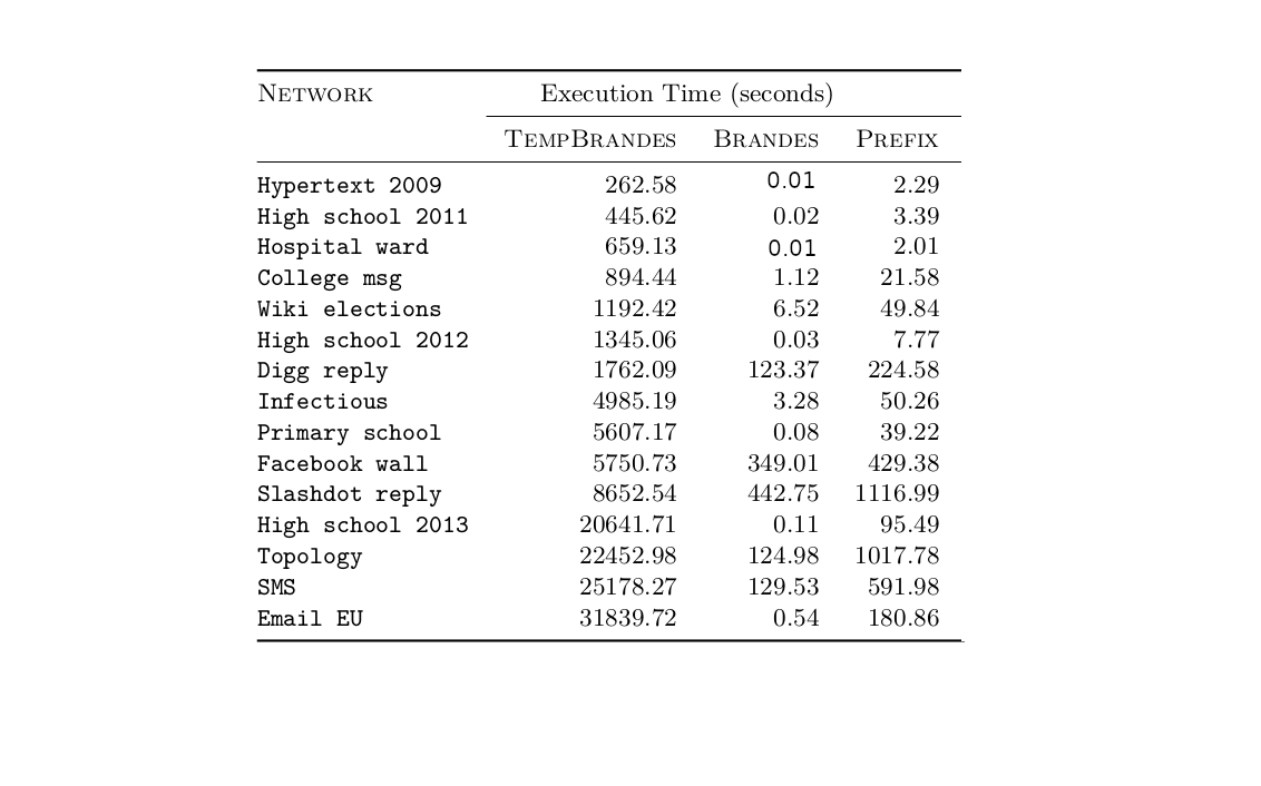
Experimental setting: temporal networks
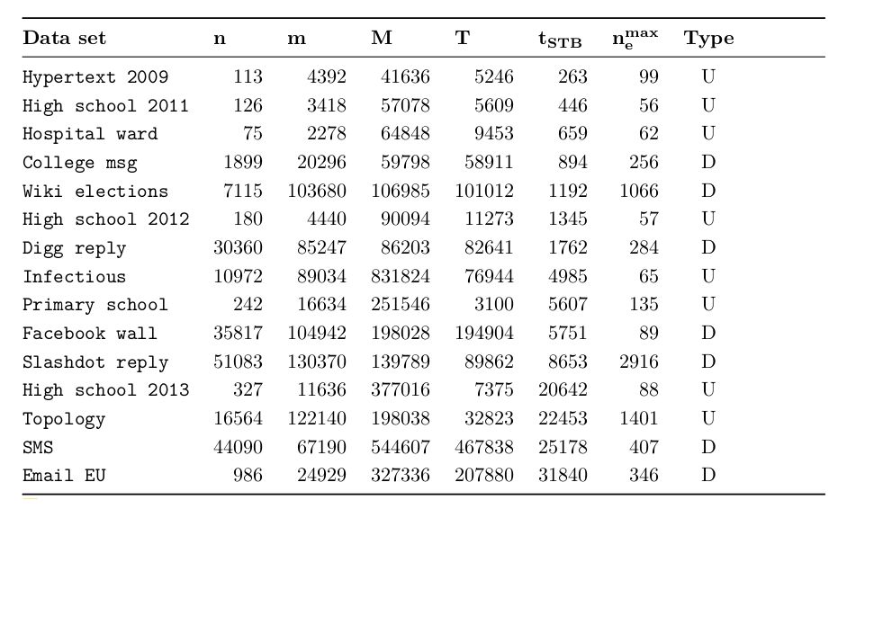
Experimental setting: implementation and evaluation
All the algorithms are implemented in Julia

- we compute a complete ranking of the nodes
- evaluate how this ranking relates to the “correct” ranking
computed by the algorithm of Bu\(\text{\ss}\) et al.
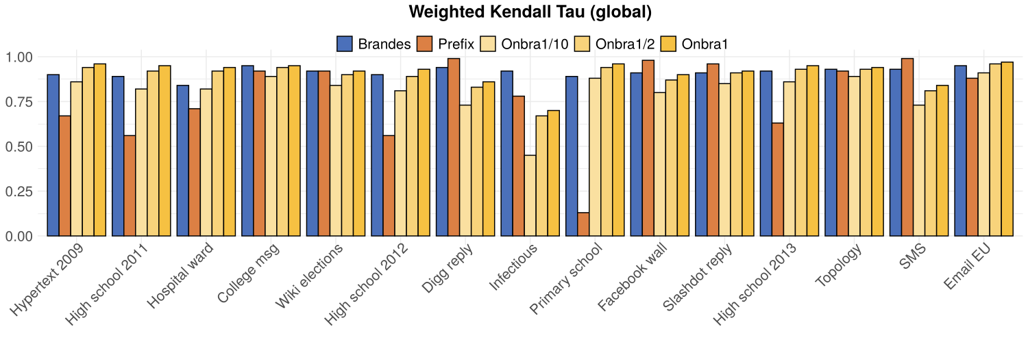
Weighted Kendall's \(\tau\) [Vigna (WWW 2015)]
TOP K nodes in the ranking
For each algorithm:
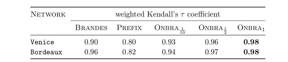
Experiment 1: global proxies (rank correlation)
Brandes
Prefix
ONBRA 1
W. Kendall's \(\tau\)
3
5
10
ONBRA \(\frac{1}{10}\)
0
11
# times a proxy wins
Experiment 1: global proxies (rank correlation)
Brandes
Prefix
ONBRA 1
W. Kendall's \(\tau\)
3
5
10
ONBRA \(\frac{1}{10}\)
0
11
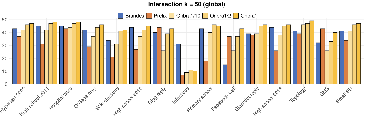
TOP(50)
2
1
12
11
3
3
# times a proxy wins
Experiment 1: global proxies (running time)
Speeding up: local proxies
Global proxies do not scale well as the network size increases!
Consider only local properties of the nodes
Neighborhood
Degree
Ego-Betweenness
A novel temporal degree notion: Pass-Through Degree
Existing temporal degree definitions:
- Degree on the underlying graph: \(d_{und}(v) = \left| \bigcup_{t\in[T]}N_t(v)\right|\)
- Average degree [Latapy (2018)]: \(d_{avg}(v) =\frac{1}{|T|}\sum_{t\in[T]}|N_t(v)|\)
Why PTD?
- \(\text{t-ptd}(v) = \sqrt{|\{(u,w)\in (V\setminus \{v\})^2\}|: u\rightarrow v\rightarrow w\}|}\)
Can be computed in \(\mathcal{O}(|\mathcal{A}|\log |A|) = \tilde{\mathcal{O}}(|\mathcal{A}|)\) time using \(\mathcal{O}(|V|+|A|)\) space
Pass-Through Degree:
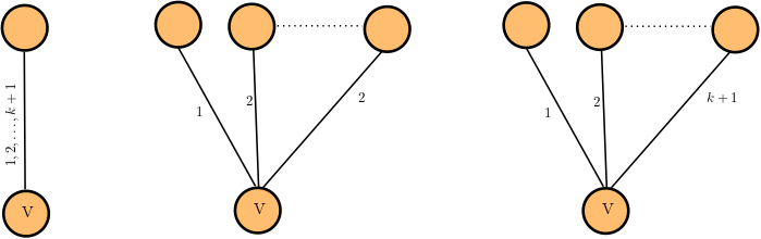
\(d_{und}(v)\)
\(d_{avg}(v)\)
\(\text{t-ptd}(v)\)
\(k+1\)
\(1\)
\(\sqrt{k}\)
\(1\)
\(1\)
\(1\)
\(k+1\)
\(1\)
\(\sqrt{\frac{k(k+1)}{2}}\approx k\)
\(N_t(v) = \{u\in N(v):(v,u,t)\in \mathcal{A}\}\)
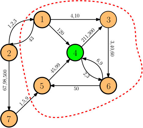
Ego Betweenness
The temporal ego-betweenness of \(u\) is the temporal betweenness computed on the temporal graph induced by the in- and out-neighbors of \(u\)
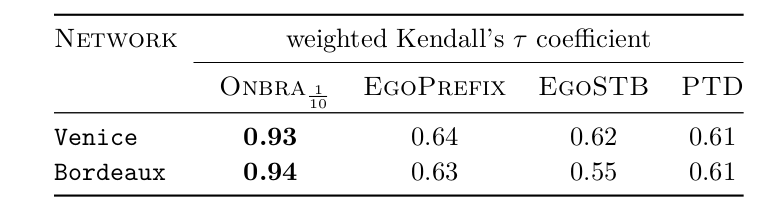
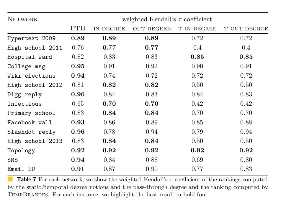
Experiment 2: local proxies (rank correlation)
W. Kendall's \(\tau\)
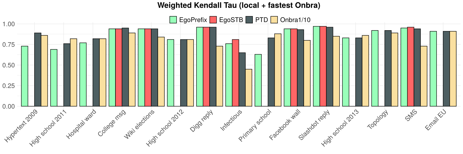
- PTD does not perform worse than EgoSTB and ONBRA
- At least as good as ONBRA on 10 over 15 networks
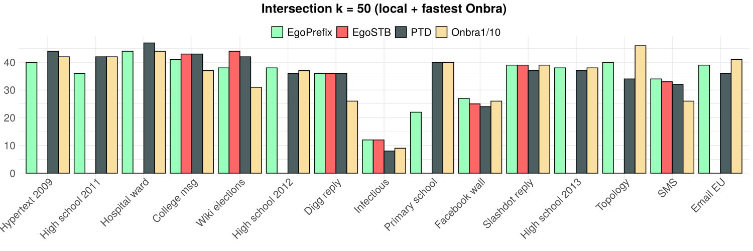
and TOP(50)
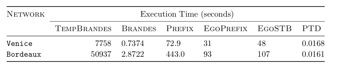
Experiment 2: local proxies (running time)
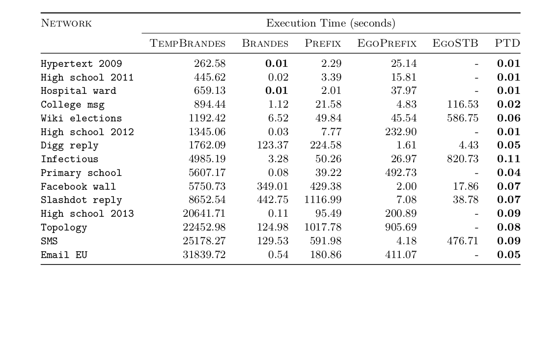
Experiment 2: local proxies (running time)
Summary of the experiments
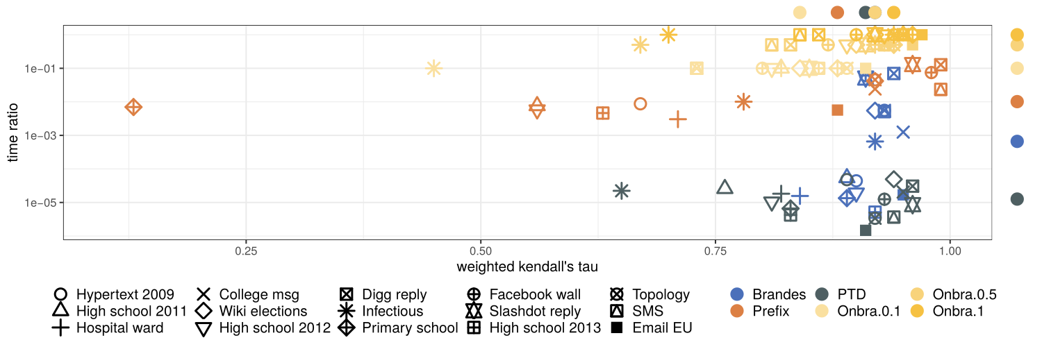
Median w. Kendalls' \(\tau\)
Median time ratio (proxy/exact)
Conclusion
In this work:
- Experimentally compared three global and three local proxies for shortest temporal betweenness
- Introduced a novel temporal degree notion
Future directions:
- Explaining the correlation between PTD and STB by using temporal graph parameters [Tang et al. (2009), Nicosia et al. (2013)]
- Use PTD as a proxy for static/temporal centrality in the context of routing schemes
- Conditional lower bound on the time complexity of computing STB
- Coditional lower bound (or better algorithm) for the ego betweenness
- Generalize the PTD to \(k\)-hop paths
Thank you

Our GitHub code
Additional experiments: other degrees as proxy
Additional experiments: transport networks
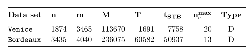
[Kujala et al. (2018)]
Additional experiments: transport networks