On the Temporal Betweenness Centrality

Antonio Cruciani
antonio.cruciani@gssi.it
Temporal Networks
Graphs are ubiquitous
they evolve over time
many of them share a common feature:

Social
Biological
Transport
....
....
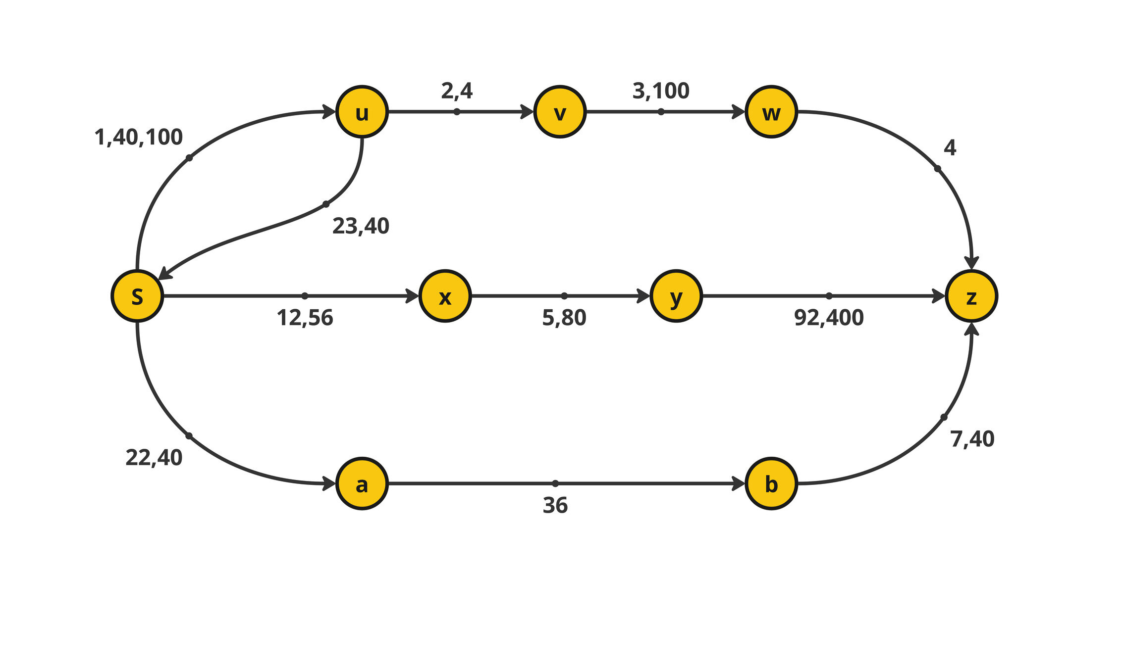
A temporal graph is an ordered triple \(\mathcal{G} = (V,\mathcal{E}, T) \), where:
- \(V\) is the set of nodes
- \(\mathcal{E}=\{(u,v,t):u,v\in V\land t\in [T]\}\) is the set of temporal edges
- \(T =\{1,2,\dots,|T|\}\) is a set of time steps
Temporal Graph
Temporal Networks
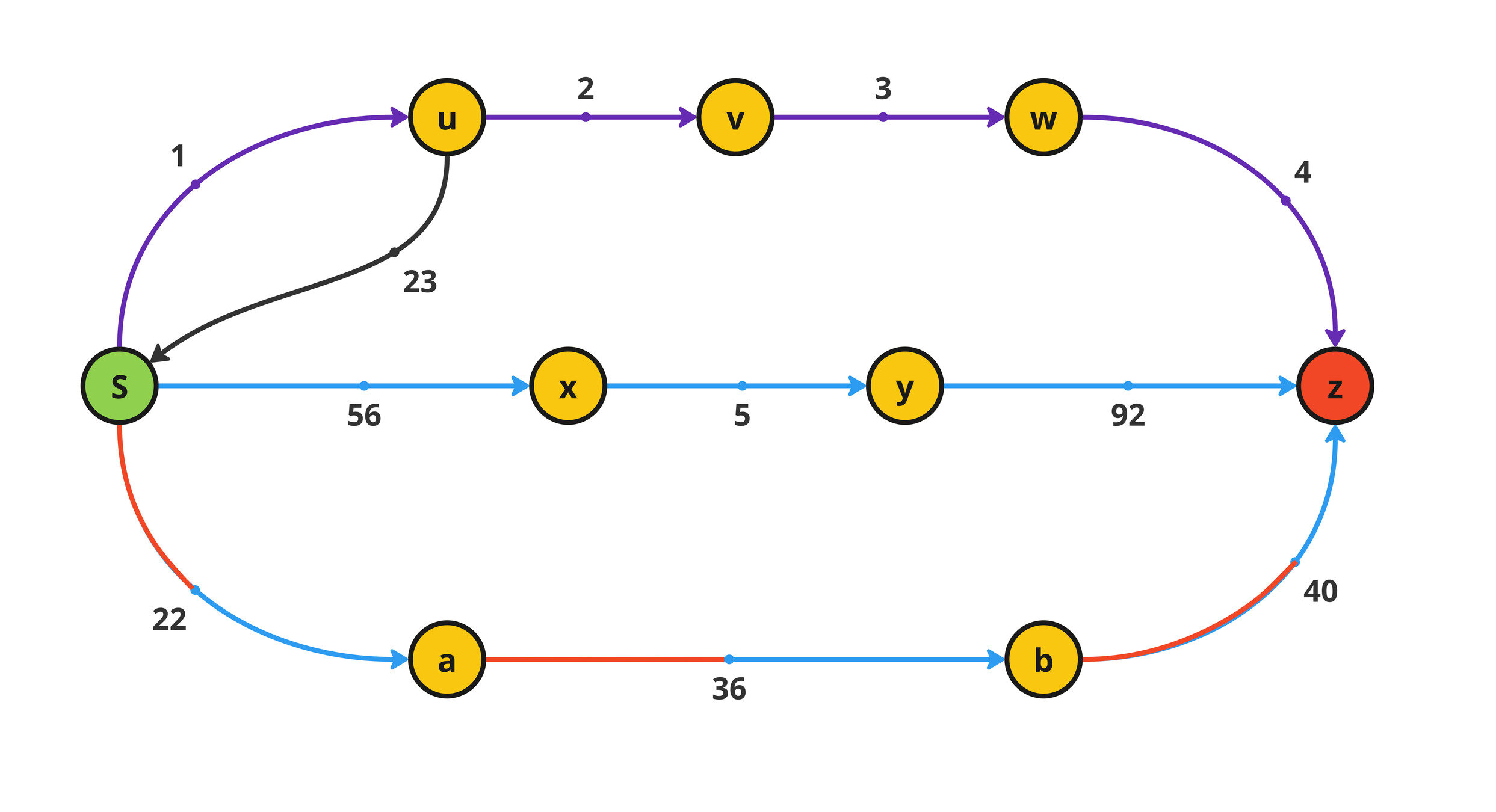
Temporal Paths
A temporal path is a sequence \(P = \langle (u_1,v_1,t_1),(u_2,v_2,t_2),\dots ,(u_k,v_k,t_k)\rangle\) of temporal arcs in which \(t_i < t_{i+1} \) and \(v_i = u_{i+1}\) for all \(i\in [k-1]\) and each node in \(V\) is visited at most once.
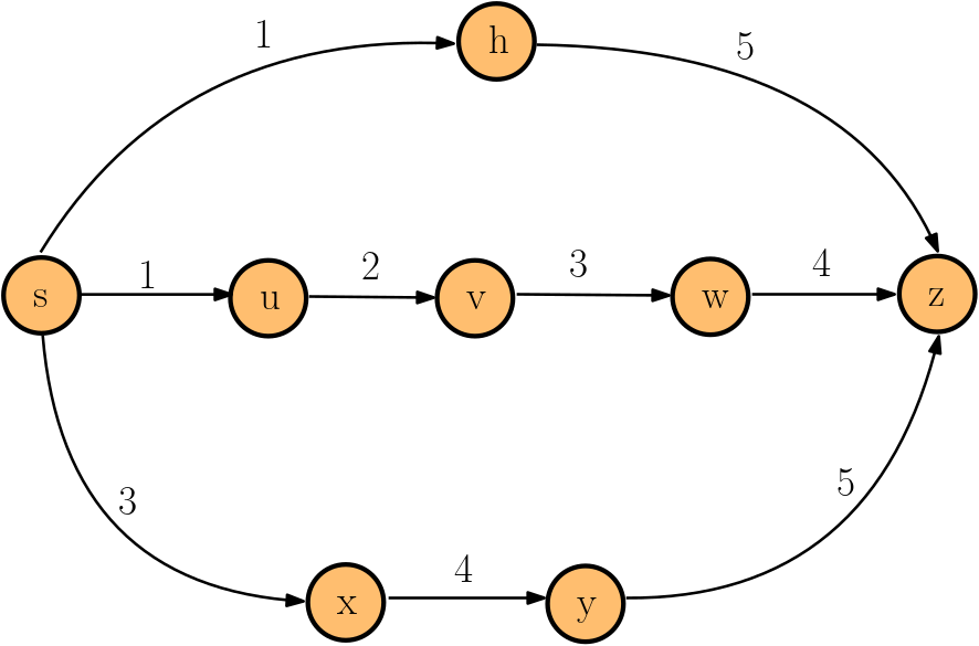
\(P = \langle s \rightarrow h\rightarrow z \rangle \)
Shortest
Foremost
Fastest
\(P = \langle s \rightarrow u \rightarrow v \rightarrow w \rightarrow z \rangle \)
\(P = \langle s \rightarrow x\rightarrow y\rightarrow z \rangle \)
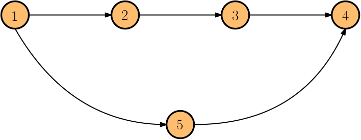
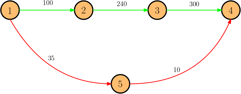
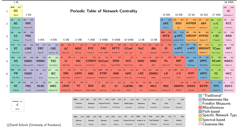
A (static) Centrality Zoo
Temporal Betweenness [Bu\(\text{\ss}\) et al (KDD 2020)]
The temporal betweeness centrality of each node \(v\in V\) is defined as
$$b^{(\star)}_v = \frac{1}{n(n-1)}\sum_{\substack{s, z\in V\\ s\neq z\neq v}} \frac{\sigma^{(\star)}_{s,z}(v)}{\sigma^{(\star)}_{s,z}}\in [0,1]$$
- \(\sigma^{(\star)}_{s,z}(v)\) is the number of \((\star)\)-temporal paths between \(s\) and \(z\) passing through \(v\)
- \(\sigma^{(\star)}_{s,z}\) overall number of \((\star\))-temporal paths between \(s\) and \(z\)
- \((\star)\) can be :
- Shortest
- Shortest-Foremost
- Prefix-Foremost
#P-Hard :(
\(\mathcal{O}(|V|^3|T|^2)\)
\(\mathcal{O}(|V| |\mathcal{E}|\log |\mathcal{E}|)\)
\(\mathcal{O}(|V||T|+|\mathcal{E}|)\)
\(\mathcal{O}(|V| + |\mathcal{E}|)\)
Time
Space
- Fastest
- Foremost
Temporal Betweenness computation
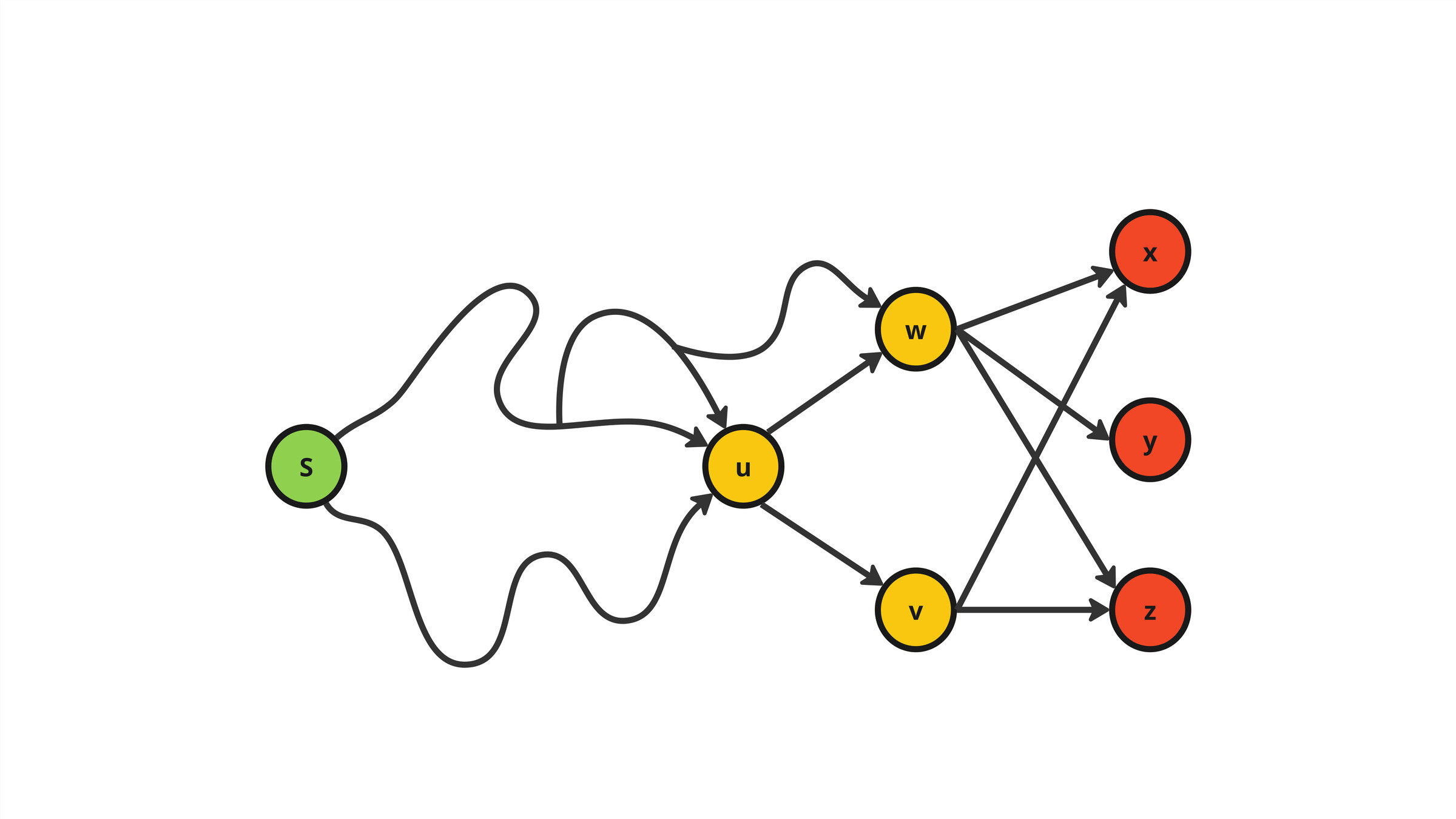
Two Pass algorithm:
For each node \(s\in V\)
- Perform a \((\star)\)-temporal BFS starting at \(s\) at time \(0\)
- Update the TBC of each (non-endpoint) node \(u\in V\) by backtracking on the DAG of the \((\star)\)-optimal temporal paths.
Step 1 (explorative step)
Some kind of modus operandi to tackle graph mining problems
Can I find a nice heuristic to ``approximate`` such a centrality measure?
Step 2 (ideal step)
Can I design a good approximation algorithm ?
Proxying Betweenness Centrality Rankings in Temporal Networks
SEA 2023
Ruben Becker,Pierluigi Crescenzi, Antonio Cruciani, and Bojana Kodric
Proxies
We say that a centrality measure \(B\) is a proxy for the centrality measure \(A\) if its ranking is "close" to the one of \(A\)
\(R_B\approx R_A\)
Here we consider one of proxy
Local
Centrality values of nodes are completely determined by the induced subgraph of their neighborhood (including themselves)
Desired properties for a proxy
Fast
Good
Ranking: list of nodes sorted in descending order of centrality value
A novel temporal degree notion: Pass-Through Degree
Existing temporal degree definitions:
- Degree on the underlying graph: \(d_{und}(v) = \left| \bigcup_{t\in[T]}N_t(v)\right|\)
- Average degree [Latapy (2018)]: \(d_{avg}(v) =\frac{1}{|T|}\sum_{t\in[T]}|N_t(v)|\)
Why PTD?
- \(\text{t-ptd}(v) = \sqrt{|\{(u,w)\in (V\setminus \{v\})^2\}|: u\rightarrow v\rightarrow w\}|}\)
Can be computed in \(\mathcal{O}(|\mathcal{E}|\log |E|) = \tilde{\mathcal{O}}(|\mathcal{E}|)\) time using \(\mathcal{O}(|V|+|E|)\) space
Pass-Through Degree:

\(d_{und}(v)\)
\(d_{avg}(v)\)
\(\text{t-ptd}(v)\)
\(k+1\)
\(1\)
\(\sqrt{k}\)
\(1\)
\(1\)
\(1\)
\(k+1\)
\(1\)
\(\sqrt{\frac{k(k+1)}{2}}\approx k\)
\(N_t(v) = \{u\in N(v):(v,u,t)\in \mathcal{E}\}\)
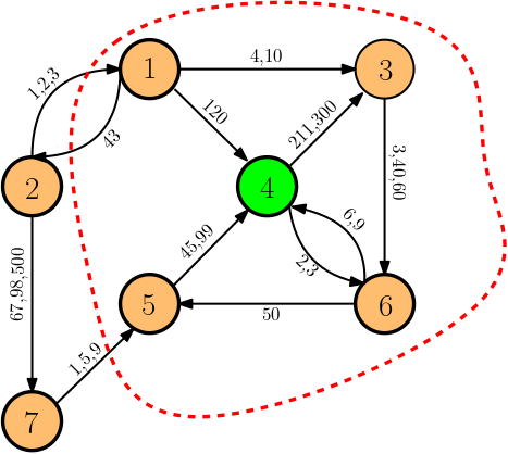
Ego Betweenness
The temporal ego-betweenness of \(u\) is the temporal betweenness computed on the temporal graph induced by the in- and out-neighbors of \(u\)
ONBRA
- Sampling-based approximation algorithm
- No Sample Complexity (stay tuned)
- For the moment let us choose a sample size such that:
- TIME(ONBRA)= \(\frac{1}{10}\)TIME(exact algorithm)
- TIME(ONBRA)= \(\frac{1}{2}\)TIME(exact algorithm)
- TIME(ONBRA) = TIME(exact algorithm)
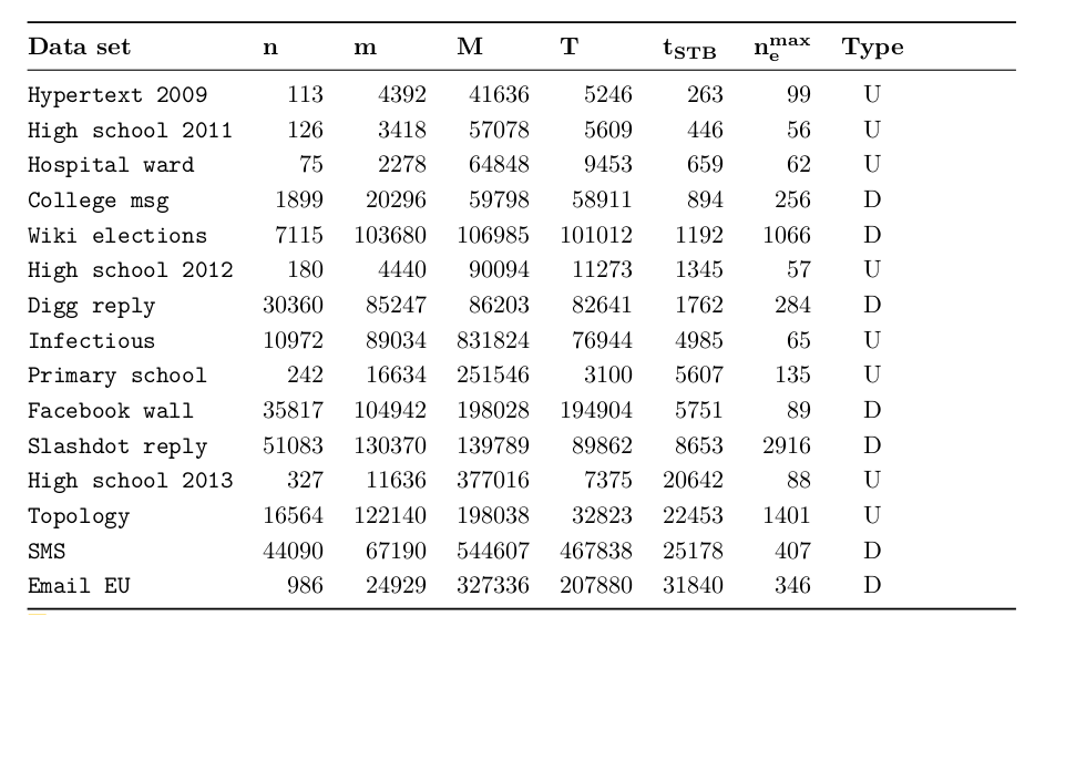
Experimental setting: temporal networks
Local proxies (rank correlation)
W. Kendall's \(\tau\)
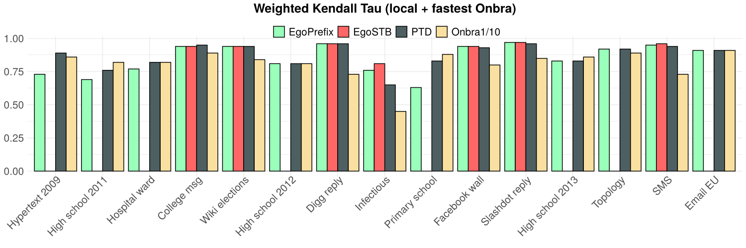
- PTD does not perform worse than EgoSTB and ONBRA
- At least as good as ONBRA on 10 over 15 networks
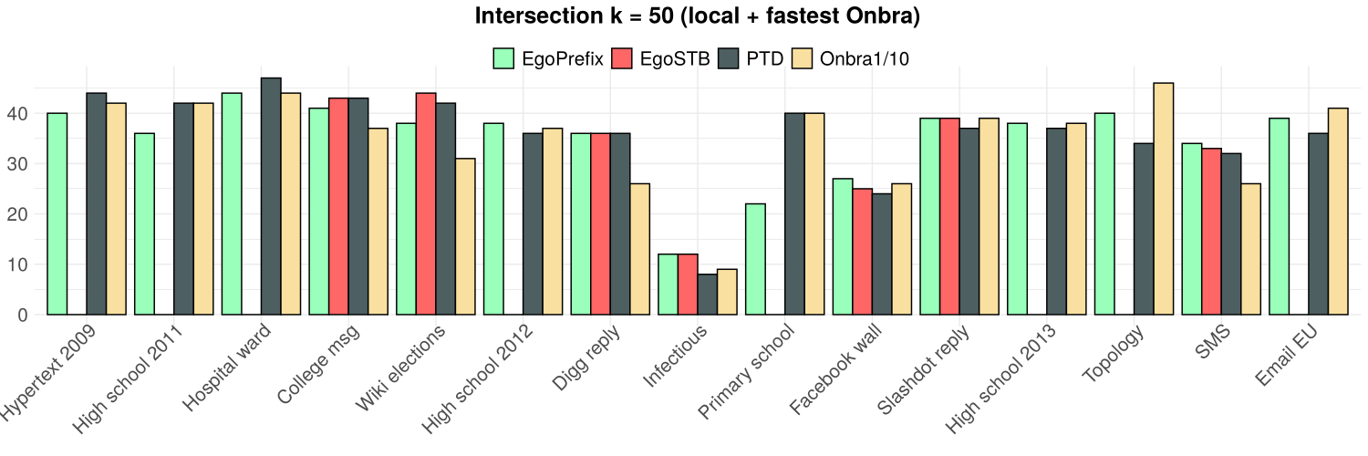
and TOP(50)
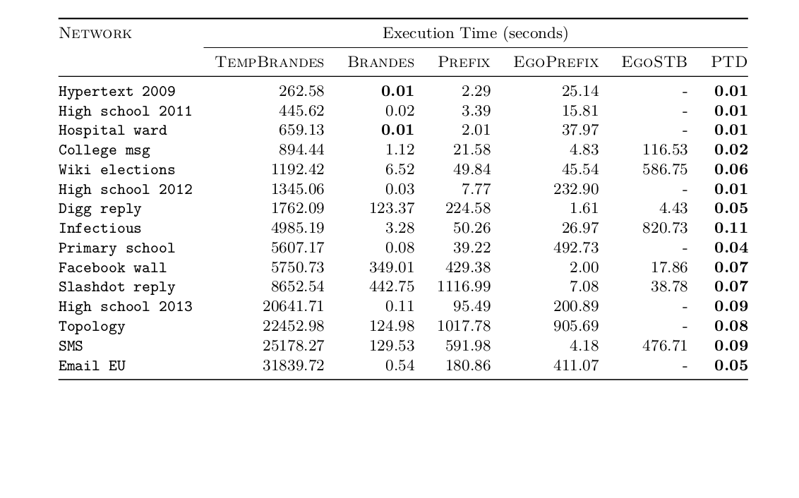
Local proxies (running time)
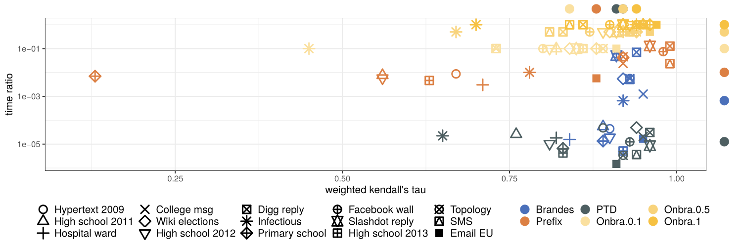
Summary of the experiments
MANTRA: Temporal Betweenness Centrality Approximation through Sampling
ECML-PKDD
2024
Antonio Cruciani
Approximating the Temporal Betweenness
$$\textbf{Pr}\left(\sup_{v\in V} \left|b_v^{(\star)}-\tilde{b}_v^{(\star)}\right|\leq \varepsilon\right)\geq 1-\delta$$
- Methods are based on random sampling to estimate the temporal betweenness centrality with an acceptable accuracy
- Problem definition:
- given \(\varepsilon,\delta \in (0,1)\) compute \((\varepsilon,\delta)\)-approximation set \(\tilde{\mathcal{B}}^{(\star)} =\{\tilde{b}_v^{(\star)}:v\in V\}\) such that
Approximating the Temporal Betweenness

How does MANTRA work?
MANTRA in three lines
- MANTRA quickly \(\text{\color{blue}``observes''}\) the temporal graph.
- MANTRA starts sampling, computing the approximation as it goes.
- At predefined intervals, MANTRA checks two stopping conditions to understand, using the sample, whether the current approximation has the desired quality.
Supremum Deviation
Given a set of functions \(\mathcal{F}\) from a domain \(\mathcal{D}\) and a sample \(\mathcal{S}\)
$$\textbf{SD}(\mathcal{F},\mathcal{S}) =\sup_{f\in \mathcal{F}}{\left| a_f(\mathcal{S})-\mu_f\right|} $$
$$a_f(\mathcal{S}) = \frac{1}{|\mathcal{S}|} \sum_{i = 1}^{|\mathcal{S}|}f(s_i) $$
$$\mu_f = \mathbb{E}[a_f(\mathcal{S})] $$
The Supremum Deviation
Goal:
$$\textbf{SD}(\mathcal{F},\mathcal{S})$$
To find an Upper bound for
Supremum Deviation
How do we estimate the SD of \(\mathcal{S}\) using a single sample?
-
\(\mathcal{S}=\)
\(\mathcal{S}=\)
-
\(\sup_{f\in\mathcal{F}}\left( a_f(\mathcal{S}_1) - a_f(\mathcal{S_2})\right)\)
\(\mathcal{S}=\)
\(\displaystyle\frac{2}{|\mathcal{S}|}\sup_{f\in\mathcal{F}}\sum_{i = 1}^{|\mathcal{S}|}\lambda_i f(z_i)\)
\(\mathcal{S}=\)
\(\mathcal{S}=\)
$$\bm{\lambda}=(\lambda_1,\lambda_2,\dots,\lambda_{|\mathcal{S}|}) \in \{-1,+1\}$$
Rademacher Averages
\(\displaystyle RA(\mathcal{F},\mathcal{S}) = \frac{1}{|\mathcal{S}|}\mathbb{E}_{\bm{\lambda}}\left[\sup_{f\in\mathcal{F}}\sum_{i = 1}^{|\mathcal{S}|}\lambda_i f(z_i)\right]\)
\(\mathcal{S}=\)
\(\mathcal{S}=\)
$$\bm{\lambda}=(\lambda_1,\lambda_2,\dots,\lambda_{|\mathcal{S}|}) \in \{-1,+1\}$$
Rademacher Complexity captures the idea of the previous slide by considering the expectation of the last formula with respect to the random choice of \(\bm{\lambda}\)
\(\displaystyle SD(\mathcal{F},\mathcal{S}) \leq 2\mathbb{E}_{\mathcal{S}\sim\mathcal{D}_r}\left[RA(\mathcal{F},\mathcal{S})\right]+\sqrt{c\frac{2\ln (2/\delta)}{r}}\)
Rademacher Averages
c-Monte Carlo Emprical Rademacher Averages (c-MCERA)
$$\bm{\lambda} \in \{-1,+1\}^{c\times|\mathcal{S}|}, r = |\mathcal{S}|$$
$$R^c_{r}(\mathcal{F},\mathcal{S},\bm{\lambda}) = \frac{1}{c}\sum_{j=1}^c \sup_{f\in\mathcal{F}}\frac{1}{r} \sum_{s_i\in\mathcal{S}}\lambda_{j,i} f(s_i) $$
With Probability at least
$$1-\delta$$
$$\mathcal{W}_\mathcal{F}(\mathcal{S})= \sup_{f\in \mathcal{F}} \frac{1}{r}\sum_{s_i\in\mathcal{S}}(f(s_i))^2$$
Empirical
Wimpy Variance
\(R = \tilde{R} + \frac{\ln(4/\delta)}{r}+\sqrt{\left(\frac{\ln(4/\delta)}{r}\right)^2 + \frac{2\ln(4/\delta)\tilde{R}}{r}}\)
\(\xi = 2R + \sqrt{\frac{2 \ln(4/\delta)\left(\hat{v}+4R\right)}{r}}+\frac{\ln(4/\delta)}{3r}\)
$$\textbf{SD}(\mathcal{F},\mathcal{S})\leq \xi$$
Variance Dependent Bound
\(\tilde{R} = R^c_{r}(\mathcal{F},\mathcal{S},\bm{\lambda}) + \sqrt{\frac{4 \mathcal{W}_{\mathcal{F}}(\mathcal{S})\ln(4/\delta)}{cr}}\)
Back to the Temporal Betweenness
\(f_v(s,z) =\frac{\sigma^{(\star)}_{s,z}(v)}{\sigma^{(\star)}_{s,z}}\)
\(\mathcal{D} = \{(s,z)\in V\times V : s\neq z\}\)
$$\tilde{b}^{(\star)}_v =\frac{1}{|\mathcal{S}|}\sum_{(s,z)\in \mathcal{S}} f_v(s,z) $$
Functions
Domain
Sample Mean
$$\mathcal{W}_\mathcal{F}(\mathcal{S})= \sup_{v\in V} \frac{1}{|\mathcal{S}|}\sum_{(s,z)\in\mathcal{S}}(f_v(s,z) )^2$$
Emp. Wimpy Variance
RTB
\(\displaystyle f_v(s) =\frac{1}{n(n-1)}\sum_{z\neq s}\frac{\sigma^{(\star)}_{s,z}(v)}{\sigma^{(\star)}_{s,z}}\)
Sample \(s\) u.a.r. from \(V\)

Perform a full temporal BFS from \(s\)
T-RK
Sample \(s\neq z\) u.a.r. from \(V\)
- Compute all the temporal paths from \(s\) to \(z\)
- Pick a temporal path \(tp_{sz}\) u.a.r.
- Increase by \(1\) the tbc of the all the nodes in \( \textbf{Int}(tp_{sz}) \)
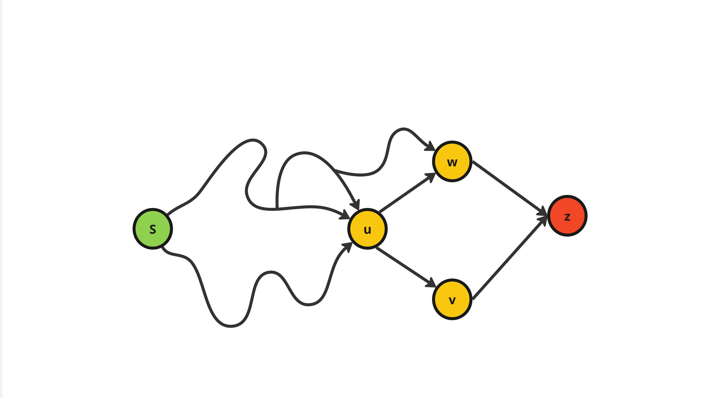
ONBRA
Sample \(s\neq z\) u.a.r. from \(V\)
- Compute all the temporal paths from \(s\) to \(z\)
- Update the temporal betweenness of all the nodes in the DAG with

\(f_v(s,z) =\frac{\sigma^{(\star)}_{s,z}(v)}{\sigma^{(\star)}_{s,z}}\)
Fact about the estimators
How many samples?
Given \(\varepsilon,\delta \in (0,1)\)
Union Bound + Hoeffding's Bound
\(\displaystyle\left|\mathcal{S}\right| = \frac{1}{2\varepsilon^2} \log\left(\frac{2n}{\delta}\right)\)
\(\textbf{SD}(\mathcal{F},\mathcal{S})\leq \varepsilon\) with probability \(\geq 1-\delta\)
How many samples?
Given \(\varepsilon,\delta \in (0,1)\)
Maximum number of nodes in the \((\star)\)-temporal optimal path
Vapnik–Chervonenkis (VC) Dimension
\(\displaystyle\left|\mathcal{S}\right| = \frac{0.5}{\varepsilon^2} \left(\lfloor \log D^{(\star)}-2\rfloor+1+\ln\left(\frac{1}{\delta}\right)\right)\)
\(\textbf{SD}(\mathcal{F},\mathcal{S})\leq \varepsilon\) with probability \(\geq 1-\delta\)
How many samples?
Given \(\varepsilon,\delta \in (0,1)\)
\(\displaystyle\left|\mathcal{S}\right|\in \mathcal{O}\left(\frac{\hat{v}+\varepsilon}{\varepsilon^2}\ln\left(\frac{\rho^{(\star)}}{\delta\hat{v}}\right)\right) \)
\(\max_{v\in V}\textbf{Var}(\tilde{b}^{(\star)}_v) \leq \hat{v}\)
\(\displaystyle \frac{1}{n(n-1)}\sum_{s,z\in V}\left|\textbf{Int}(tp_{sz})\right| \)
Variance-Aware
\(\textbf{SD}(\mathcal{F},\mathcal{S})\leq \varepsilon\) with probability \(\geq 1-\delta\)
Another challenge!
How do we compute \(\rho^{(\star)}\)?
All-Pairs \((\star)\)-Temporal Paths
\(\mathcal{O}(|V||\mathcal{E}|\)) :((
Let's use sampling to approximate these values !!!
Fast Approximation of \(D^{(\star)}\) and \(\rho^{(\star)}\)
Very high-level idea
With a sample of \(k=\Theta\left(\frac{\ln n}{\varepsilon^2}\right)\) nodes, we can approximate w.h.p.
- \(\rho^{(\star)}\) with the absolute error bounded by \(\varepsilon \frac{D^{(\star)}}{\zeta}\)
- \(D^{(\star)}\) with the absolute error bounded by \(\frac{\varepsilon} {\zeta}\)
- \(\zeta\) with the absolute error bounded by \(\varepsilon\)
Perform \(k\) \((\star)\)-Temporal BFS from random nodes
Temporal Connectivity Rate
MANTRA
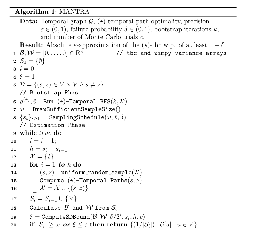


Bootstrap Phase
Estimation Phase
Experimental Setting

All the algorithms have been implemented in Julia
Every algorithm is run 10 times
\(\delta = 0.1\)
\(\varepsilon\in\{0.1,0.07,0.05,0.01,0.007.0.005,0.001\}\)
Parameters:
\(c = 25\)
Machine used: Server with Intel Xeon Gold 6248R (3.0GHz)
32 cores and 1TB RAM thank you CySTAR :)
Temporal Networks
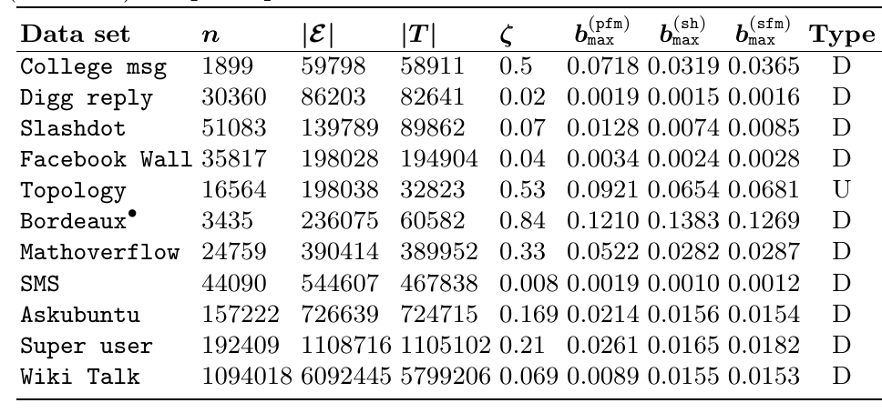
Temporal Networks: properties
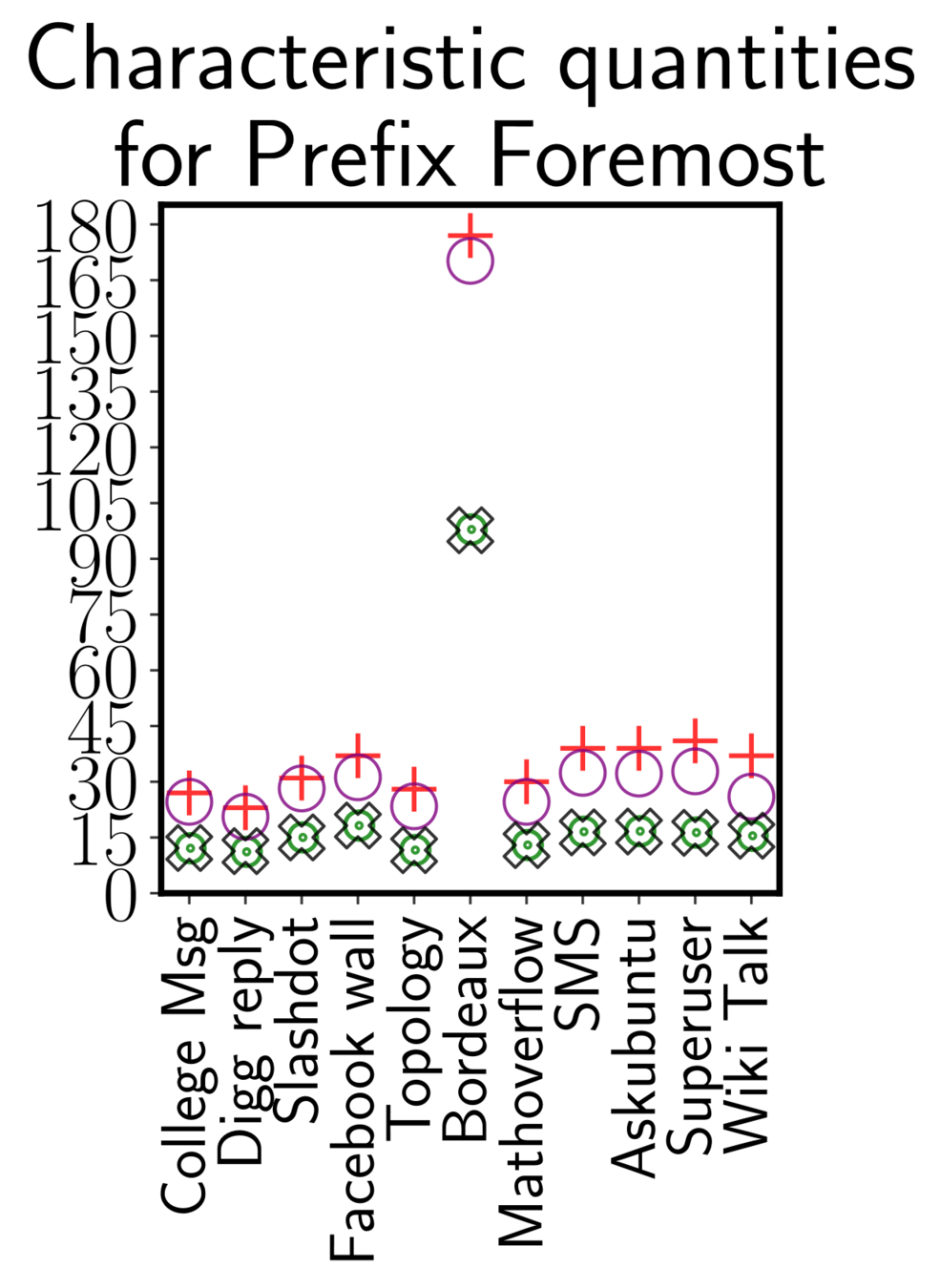
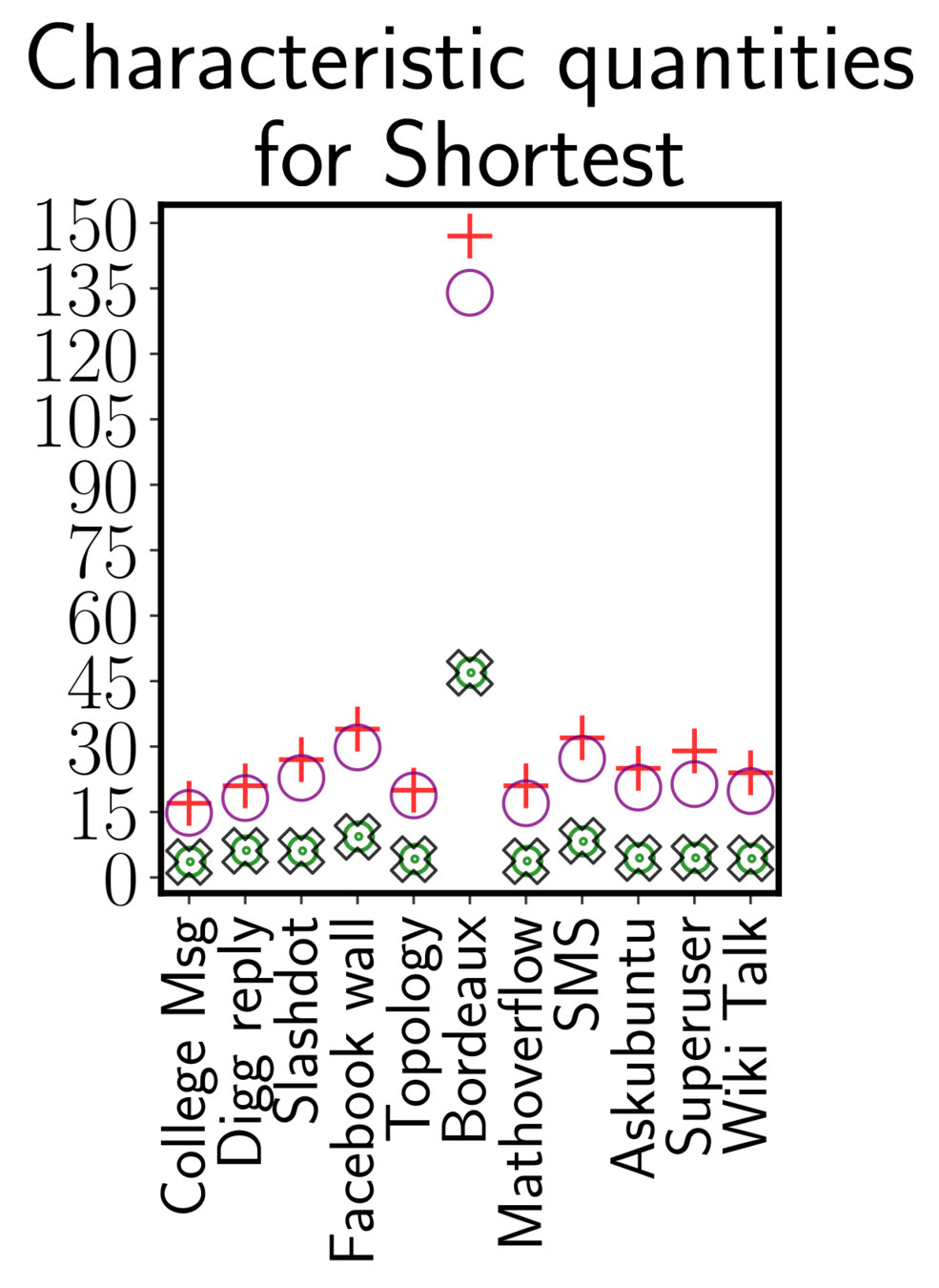
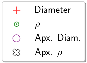
Running time sampling algorithm
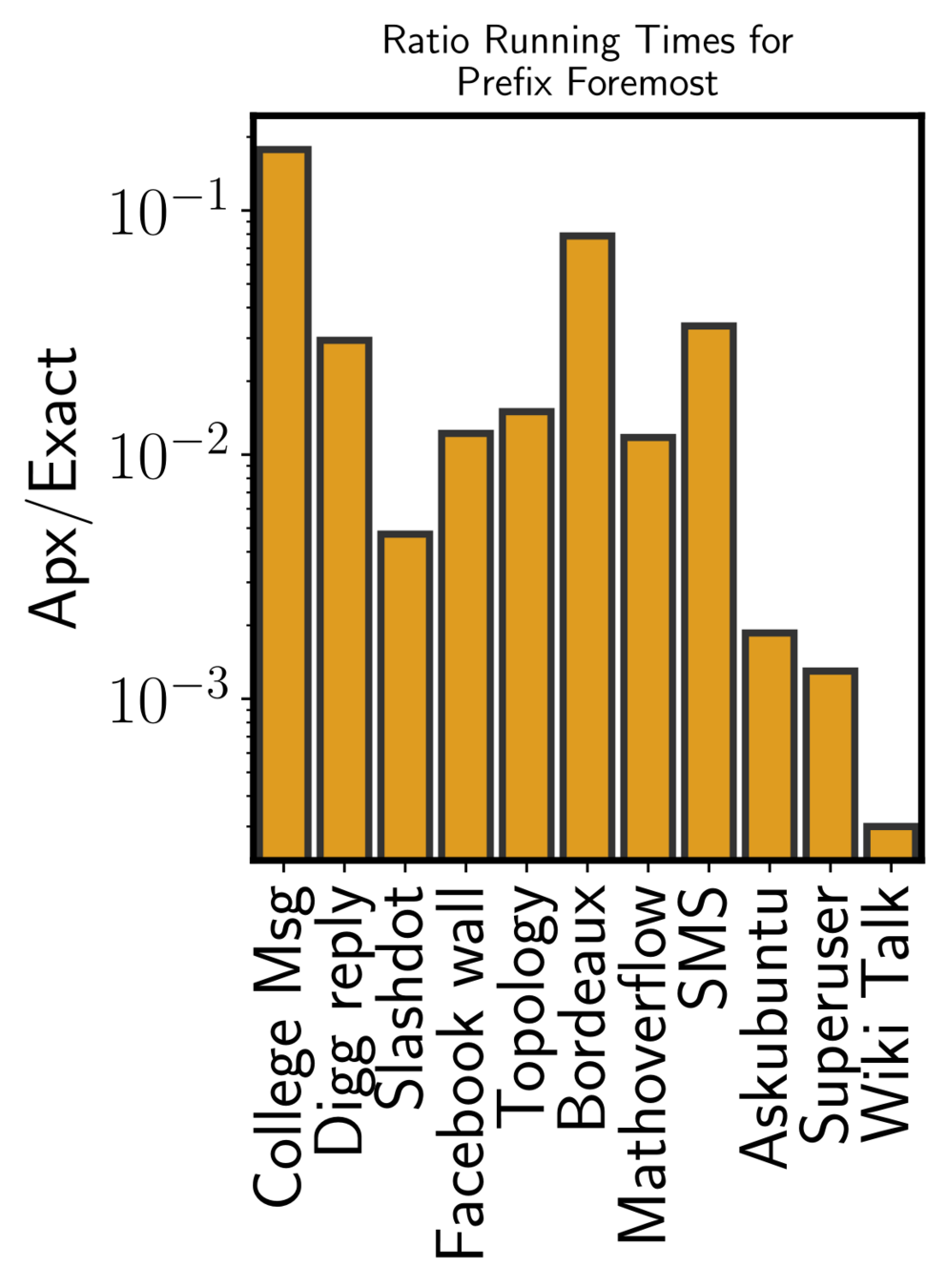
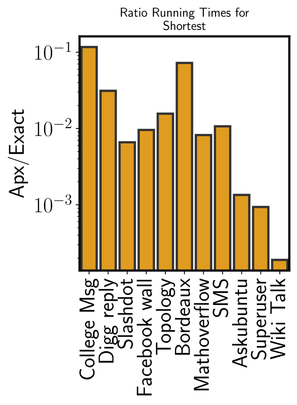
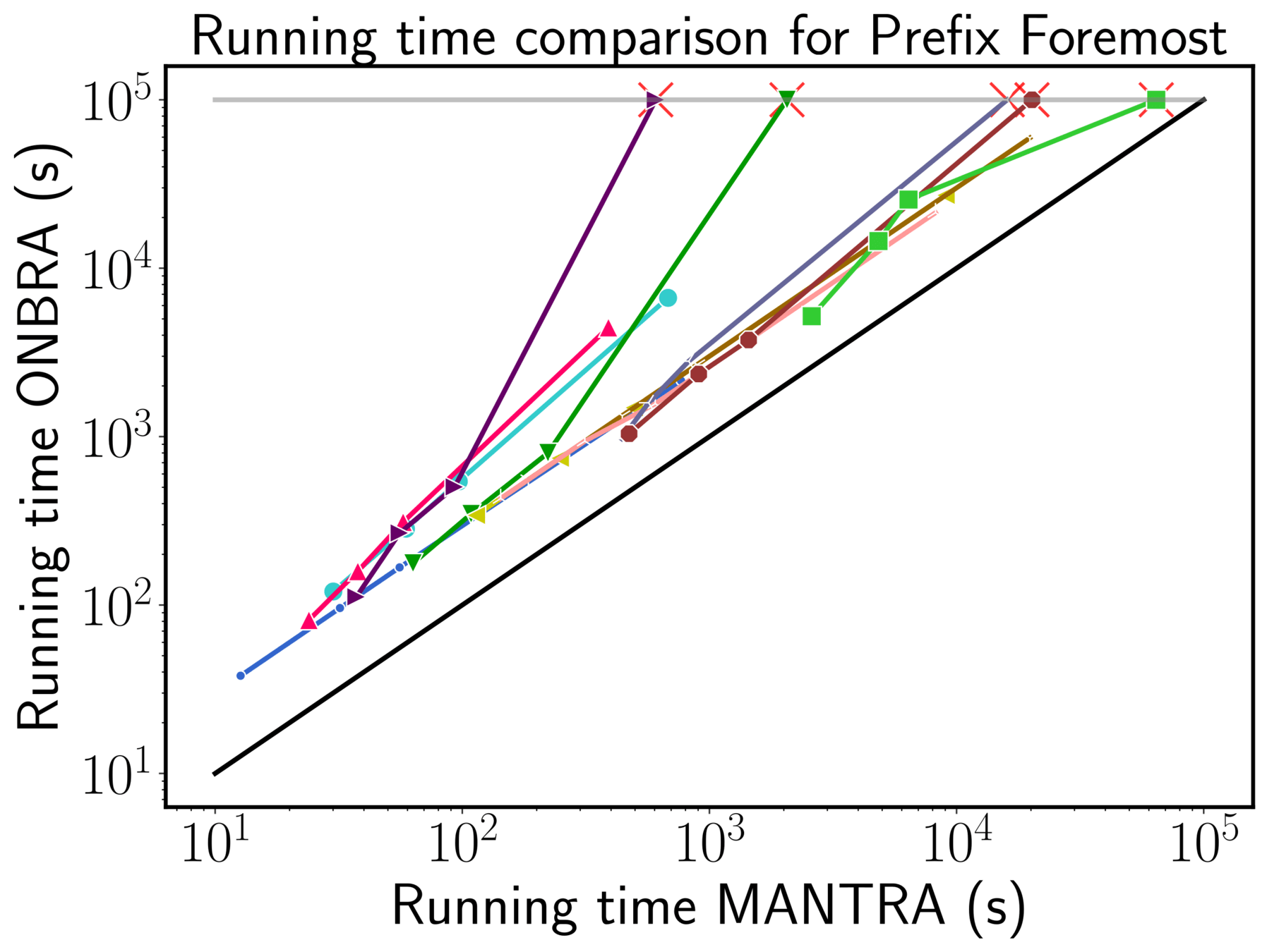

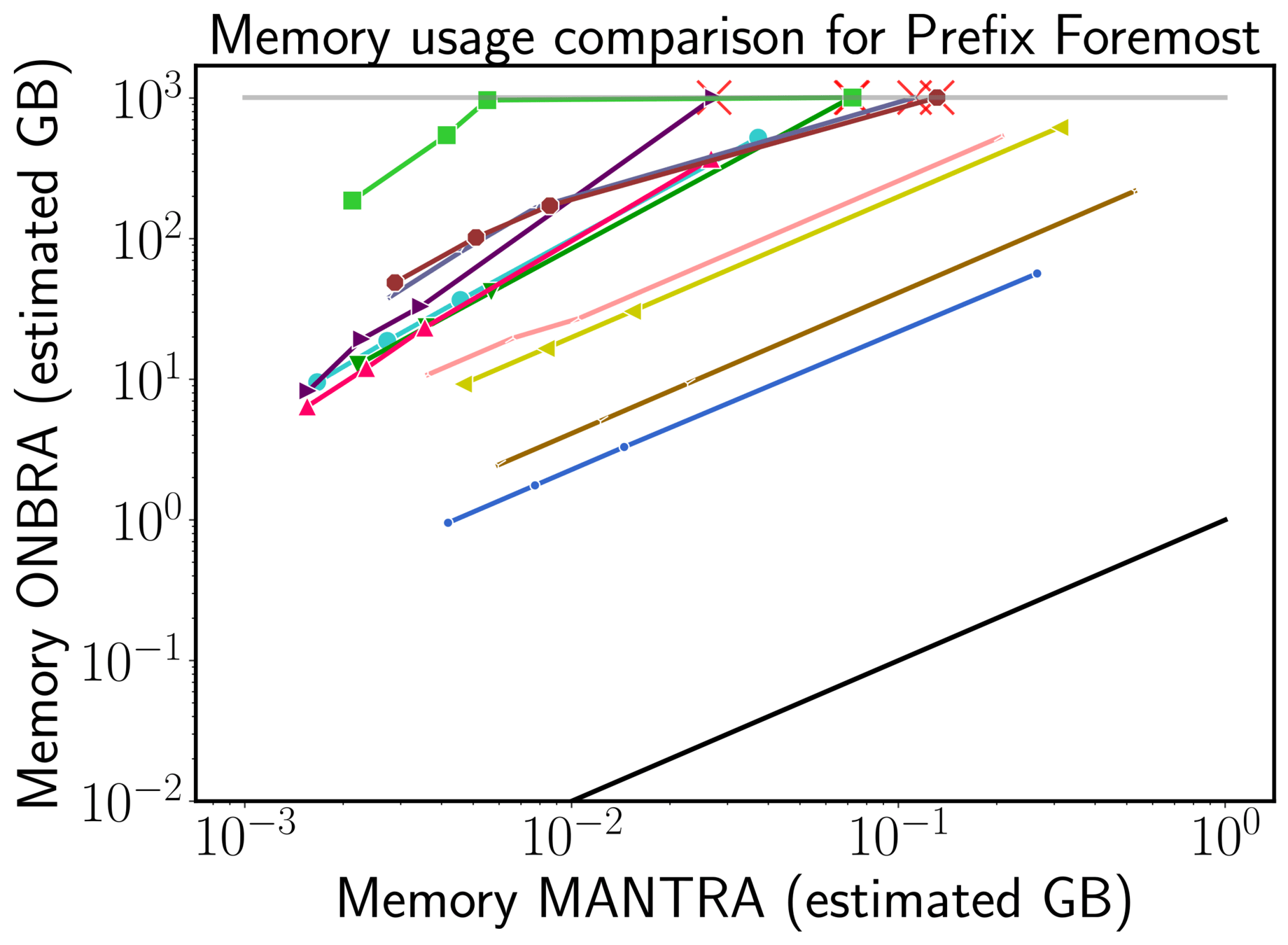
ONBRA needs more than 1TB of RAM!!!
Speed an Sample size MANTRA vs ONBRA
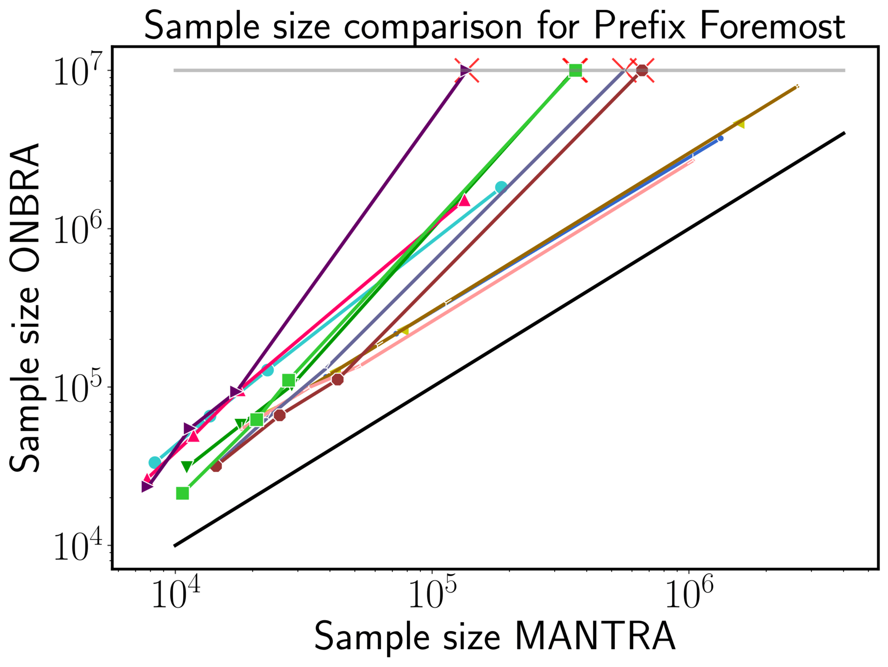

Space MANTRA vs ONBRA
Conclusions
- Introduced MANTRA, a novel sampling-based approximation algorithm for the temporal betweenness centrality
- Provided a sample-complexity analysis for the temporal betweenness estimation problem
- Provided a sampling-based approximation algorithm for temporal distance-based metrics in temporal graphs
- Theoretically and experimentally showed the advantage of using our framework over the state of the art
Future directions
- Use the novel temporal graph traversal proposed by Brunelli et al. in KDD 2024 to speed-up MANTRA
- Extend MANTRA to the computation of set centralities as for the static case [Pellegrina KDD 2023]
- Use MANTRA to find communities in temporal graphs
Thank You!

MANTRA
STBProxy
