Dynamic graph models inspired by the Bitcoin network-formation process
Antonio Cruciani
Gran Sasso Science Institute (GSSI), L’Aquila, Italy
antonio.cruciani@gssi.it
Francesco Pasquale
Università di Roma ‘‘Tor Vergata’’, Rome, Italy
francesco.pasquale@uniroma2.it

In this work
- Define and analyze three dynamic random graph models inspired by the Bitcoin P2P network generation protocol
-
To understand the properties of the network
- Expansion (robustness)
- Reliability (for spreading messages)
What we do:
Why we do it:
How we do that:
- We simulate the models
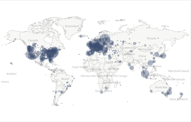
The Bitcoin P2P Network
- We can approximately retrieve the set of peers
- But we can't find the links between them
What do we know?
Every node:
- Min 8 connections
- Max 125 connections
Can we use it to model the network structure?
Some related works
-
Bitcoin topology inference:
- Miller et al. (2015), Neudecker et al. (2016), Delgado-Segura et al. (2018)
Difficult to apply on the real Bitcoin P2P Network
-
Dynamic random graph models:
- Becchetti et al.(2020) [RAES MODEL]
Dynamic graph that converges to a static random graph
We extend the RAES model
Bitcoin Topology Inference
- (Miller et al.) Discovering bitcoin’s public topology and influential nodes. 2015
- (Neudecker et al.) Timing analysis for inferring the topology of the bitcoin peer-to-peer network. 2016
- (Delgado-Segura et al.) TxProbe: Discovering Bitcoin’s Network Topology Using Orphan Transactions. 2018
Dynamic Graph Models (Inspired by the Bitcoin Network)
- (Becchetti et al.) Finding a bounded-degree expander inside a dense one. (RAES Model) 2020
E-RAES (Edge Dynamic-RAES)
Example:
n : 20
d : 4
c : 1.5
p : 0.5
At each round, each node \(u \in V\), independently of the other nodes:
- If \(u\) has degree \(\delta_u < d\), then connects to \(d-\delta_u\) new nodes.
- If \(u\) has degree \(\delta_u > c\cdot d\), then \(u\) picks \(\delta_u -(c\cdot d)\) neighbors u.a.r. and drops the connections with them.
- Every edge disappears with probability \(p\).
RAES
E-RAES: Theoretical analysis?
Non-Reversible Ergodic Markov Chain
E-RAES Process
- Mixing Time ?
- Stationary random graph properties?
- Flooding time?
Simulations
E-RAES: empirical "Steady-state" convergence
\(\mathcal{P_t} = D(\mathcal{G_t})^{-1} A(\mathcal{G_t})\)
Measure of robustness: Spectral-Gap
At every round \(t\geq 0\) compute:
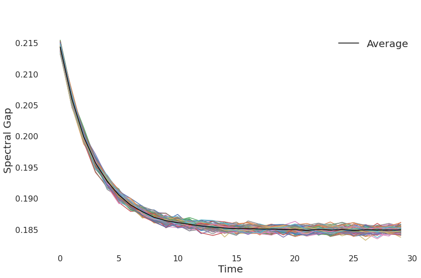
E-RAES: empirical "Steady-state" convergence
At the generic round \(t\geq \log n\):
If \(|\gamma_t - \gamma_i|\leq \varepsilon\) for each \(i \in [(t-\log n), t]\)
How do we choose \(\varepsilon\)?
- Run the process for k rounds
- Set \(\varepsilon = \frac{1}{k}\sum_{i=1}^{k} | \gamma_i - \gamma^{mean}|\)
Empirical convergence:
E-RAES: (Average) Expansion
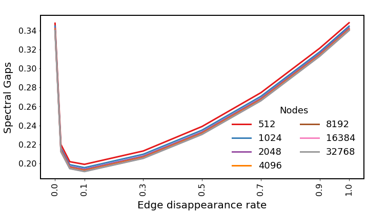
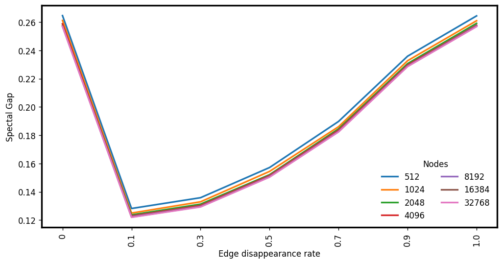
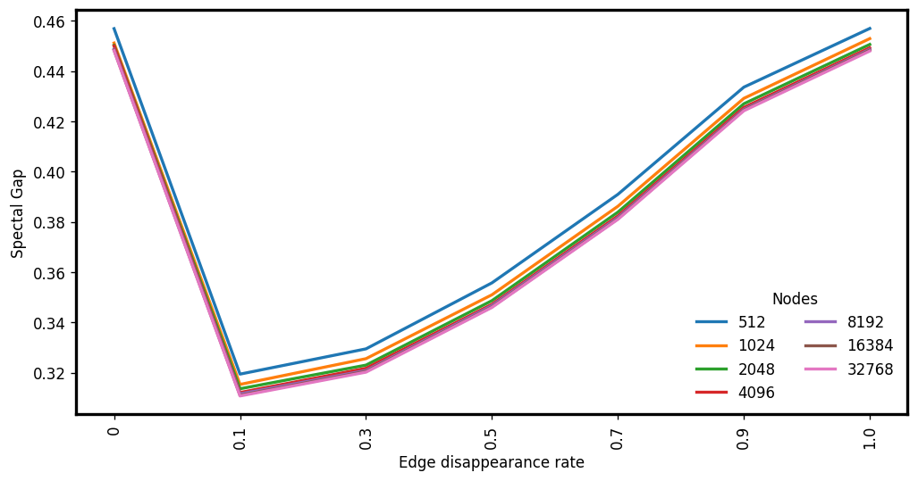
Expansion measured before the edge disappearance phase
\(d : 4, c: 1.5\)
\(d : 6, c: 5\)
\(d : 3, c: 3\)
E-RAES: (Average) Flooding Time
Flooding step executed after the edge disappearance phase
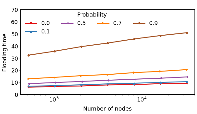
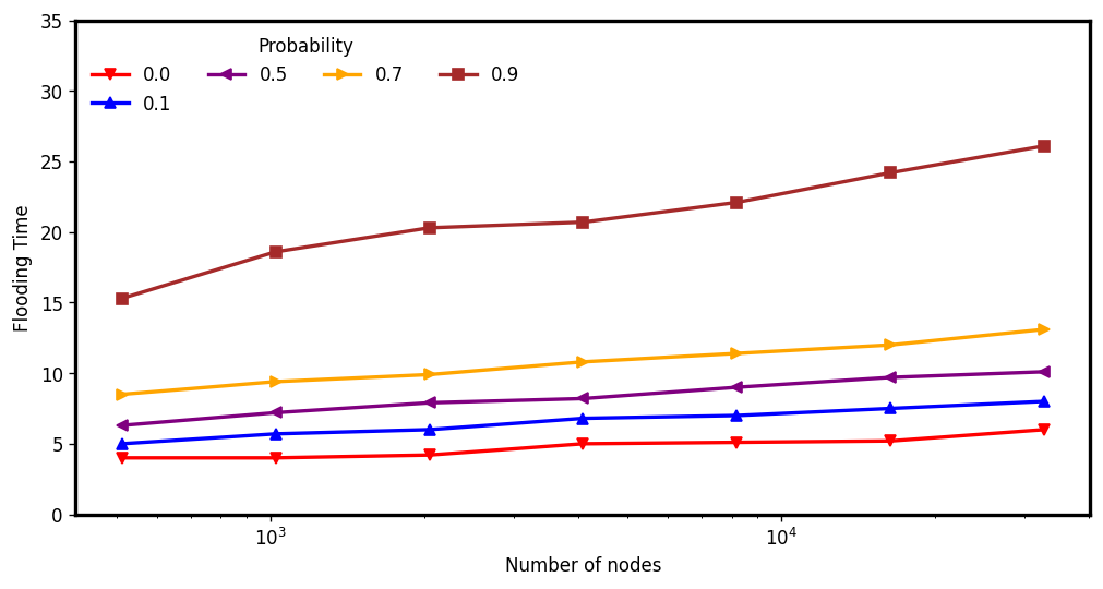
\(d : 4, c: 1.5\)
\(d : 6, c: 5\)
\(d : 3, c: 3\)
V-RAES (Vertex Dynamic-RAES)
At each round \(t\geq 0\):
- \(N_\lambda(t)\sim \text{Poisson}(\lambda)\) young nodes join the graph and connect to \(d\) random old nodes.
- If an old node \(u\) has degree \(\delta_u < d\), then connects to \(d-\delta_u\) additional old nodes.
- If an old \(u\) has degree \(\delta_u > c\cdot d\), then \(u\) picks \(\delta_u -(c\cdot d)\) neighbors u.a.r. and drops the connections with them.
- Every (young and old) node disappears with probability \(q\).
Example (ignore self-loops):
\(\lambda\) : 5
d : 4
c : 1.5
q : 0.5
V-RAES: "Steady-state" convergence
Markovian Queue
V-RAES Process
Stationary when \(|V_t| \approx \frac{\lambda}{q}\)
V-RAES: % of informed nodes at each round
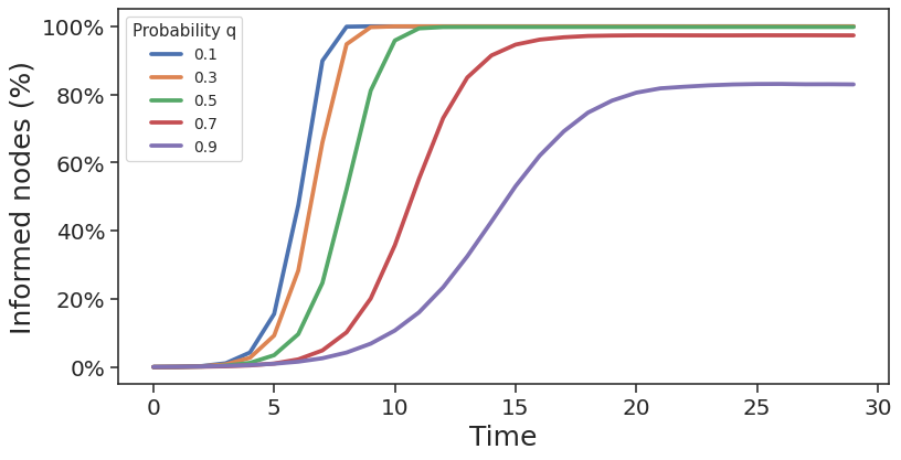
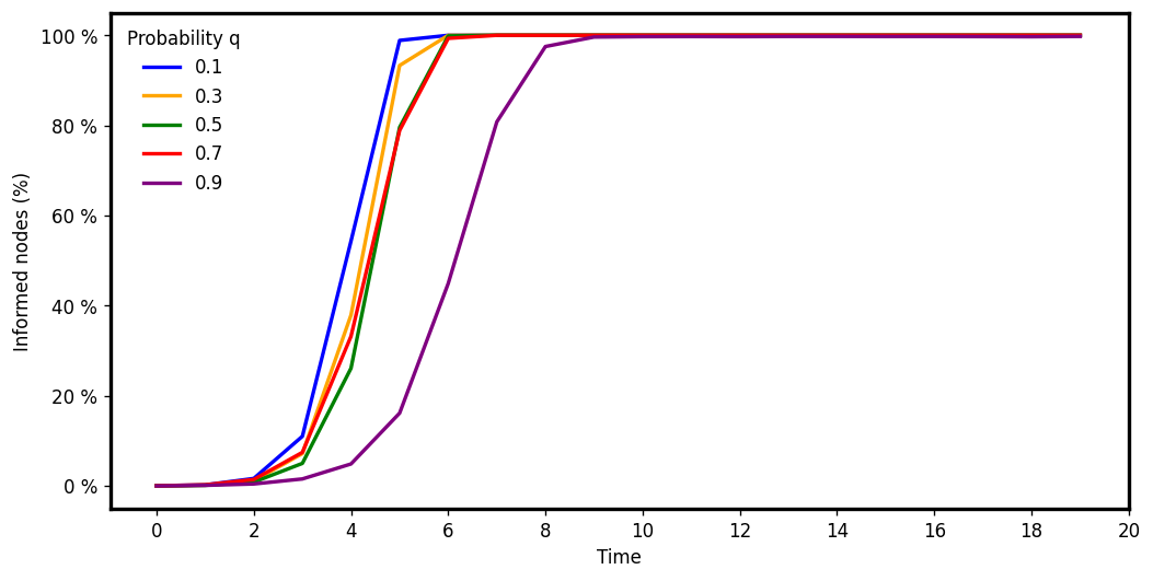
\(d : 4, c: 1.5\)
\(d : 6, c: 5\)
\(d : 3, c: 3\)
Flooding step executed after the edge disappearance phase
Network size: \(\frac{\lambda}{q} = 2^{15}\)
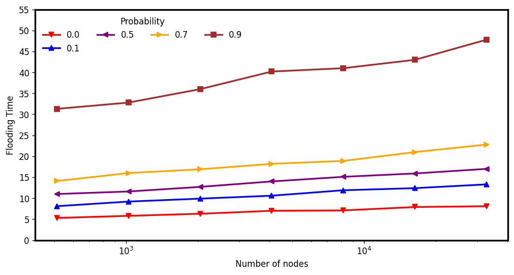
V-RAES: (Average) Flooding time
Flooding step executed after the edge disappearance phase
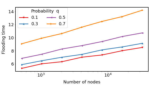
\(d : 4, c: 1.5\)
\(d : 6, c: 5\)
\(d : 3, c: 3\)
EV-RAES (Edge-Vertex Dynamic-RAES)
At each round \(t\geq 0\):
- \(N_\lambda(t)\sim \text{Poisson}(\lambda)\) young nodes join the graph and connect to \(d\) random old nodes.
- If an old node \(u\) has degree \(\delta_u < d\), then connects to \(d-\delta_u\) additional old nodes.
- If an old \(u\) has degree \(\delta_u > c\cdot d\), then \(u\) picks \(\delta_u -(c\cdot d)\) neighbors u.a.r. and drops the connections with them.
- Every (young and old) node disappears with probability \(q\).
- Every edge disappears with probability \(p\).
Example (ignore self-loops):
\(\lambda\) : 5
d : 4
c : 1.5
q : 0.5
p: 0.5
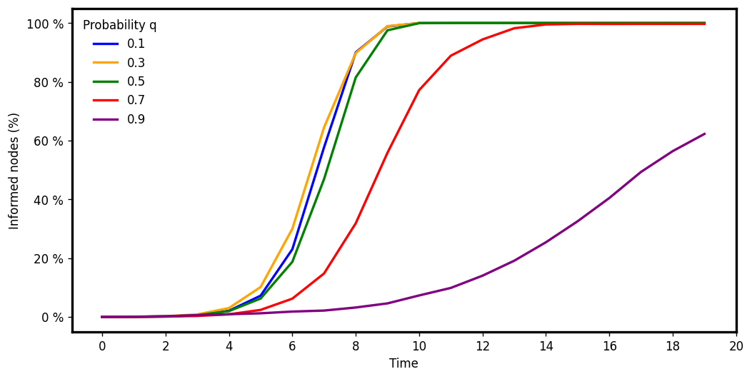
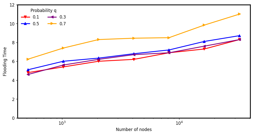
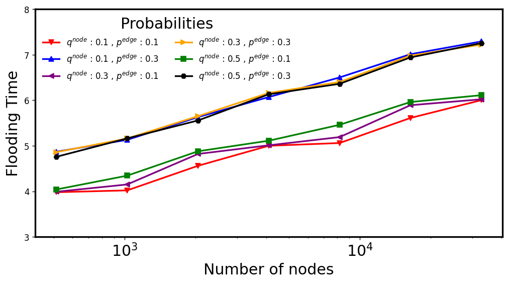
EV-RAES: Sparse vs Bitcoin default values
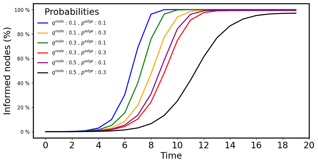
\( d: 4, c: 1.5\)
\(q\in [0.1,0.5],p\in [0.1,0.3] \)
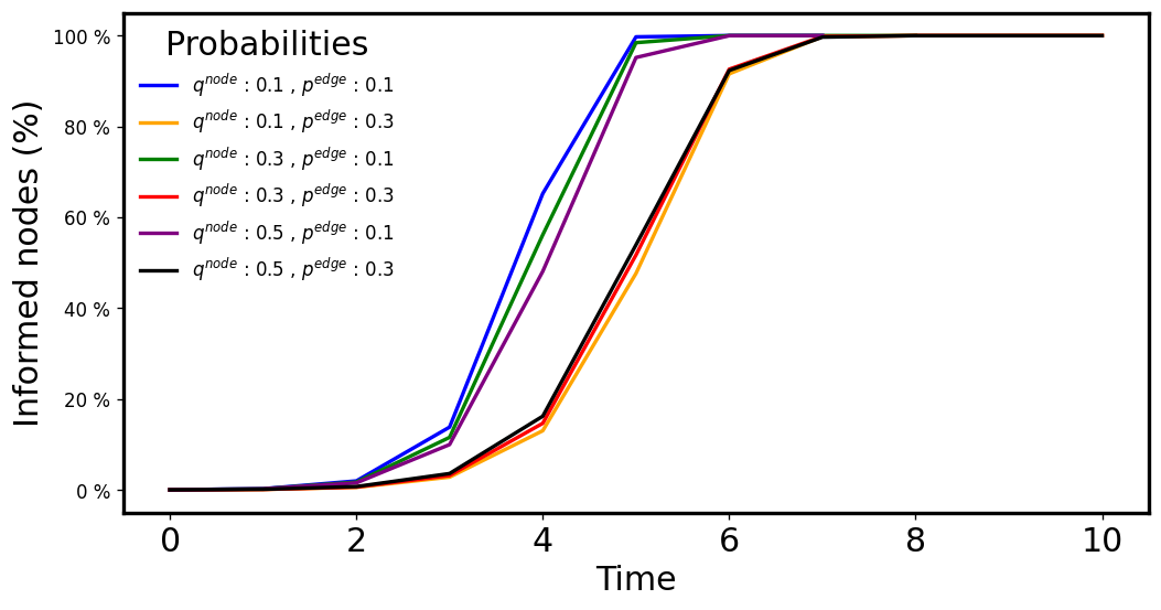
\( d: 8, c: 15.625\)
\(q\in [0.1,0.5],p\in [0.1,0.3] \)
Network size: \(\frac{\lambda}{q} = 2^{15}\)
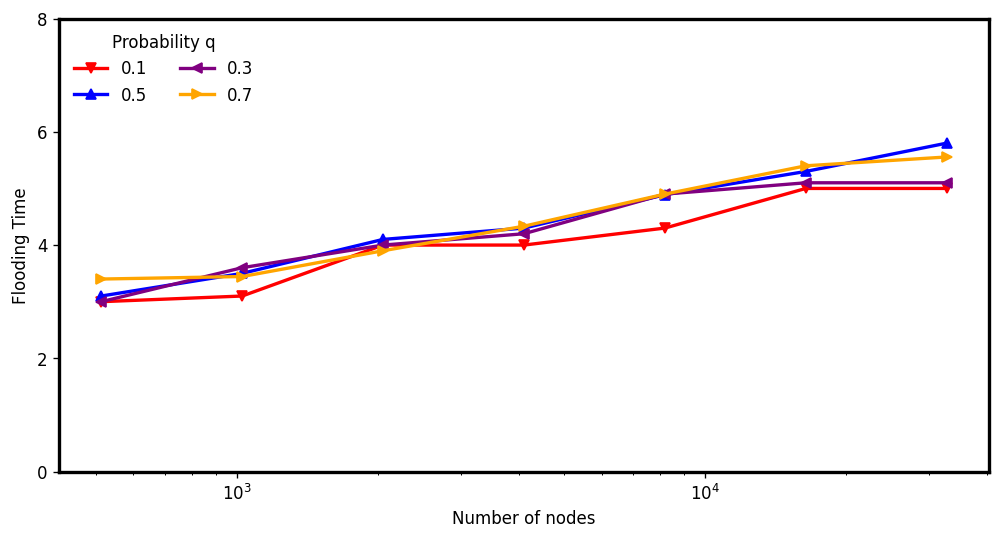
\( d: 4, c: 1.5\)
\(q\in [0.1,0.5],p\in [0.1,0.3] \)
\( d: 8, c: 15.625\)
\(q\in [0.1,0.5],p\in [0.1,0.3] \)
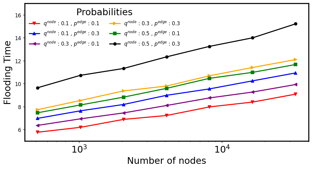
EV-RAES: Sparse vs Bitcoin default values
Conclusions and Future works
Conclusions
Future works
- E/V/EV- RAES protocols build very robust networks.
- Information Spreading in the three models is fast and reliable
- Theoretical analysis of these models?
- Study a power-law distribution model?
Thank You!